Bayesian Assurance of Consecutive Studies

J. Kyle Wathen and Laurent Spiess

June 04, 2025

The following scripts are related to the Integration Point: Analysis, the Integration Point: Response, and the Integration Point: Initialization. Click on the links for more information about these integration points.

Introduction

The intent of the following examples is to demonstrate the computation of Bayesian assurance, or probability of success, through the integration of R with Cytel products. The first example features a two-arm, fixed-sample trial with normally distributed outcomes, using a non-standard prior to compute assurance. Subsequent examples advance to more complex scenarios, including computing assurance for a sequential design involving a phase 2 trial with normal outcomes followed by a phase 3 trial with time-to-event outcomes.

All examples involve two treatments: Standard of Care (S) and Experimental (E). The scenarios covered are as follows:

1. Fixed sample design using a mixture of normal distributions to compute Bayesian assurance.
2. Group sequential design, expanding on Example 1, with an interim analysis for futility based on Bayesian predictive probability.
3. Fixed design with a time-to-event outcome, serving as both a standalone example and a reference for the later phase 2/phase 3 scenario.
4. Two consecutive studies: phase 2 with a normal endpoint followed by phase 3, also with a normal endpoint.
5. Two consecutive studies: phase 2 with a normal endpoint followed by phase 3 with a time-to-event outcome.

Once CyneRgy is installed, you can load this example in RStudio with the following commands:

CyneRgy::RunExample( "AssuranceConsecutiveStudies" )

Running the command above will load the RStudio project in RStudio.

East Workbook: AssuranceConsecutiveStudies.cywx

RStudio Project File: AssuranceConsecutiveStudies.Rproj

In the R directory of this example you will find the R files used in the examples.

Example 1 - Fixed Sample Design with a Mixture of Normal Distributions

This example considers a two-arm fixed sample design with normally distributed outcomes $Y$, with 80 patients per treatment arm. It demonstrates how to customize the Response (Patient Simulation) element of East Horizon’s simulation to simulate a mixture of normal distributions, and the Analysis element of East Horizon’s simulation to compute the probability of success.

By integrating an R function into the Analysis integration point, users can evaluate the frequentist operating characteristics of the Bayesian design in East Horizon. Additionally, by modifying the Response integration point, the simulation will incorporate Bayesian assurance. Specifically, an R function first samples from the assurance prior, then generates the patient data. The resulting power from this simulation reflects the Bayesian assurance, assuming the two-component prior.

Often, it is important to examine the posterior distributions of both the observed and true treatment differences following a Go decision. These posterior distributions provide valuable insights for planning subsequent study phases and assessing potential risks. The process of obtaining these posterior distributions is detailed in the next example, and their application to Phase 2 and Phase 3 studies is explored in later sections.

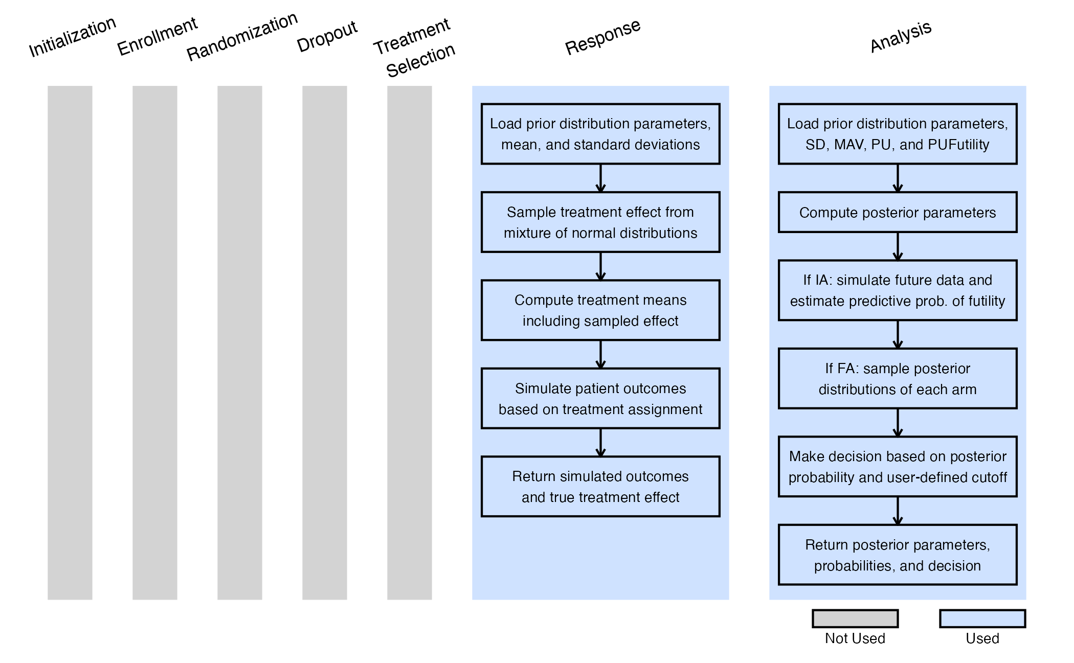
The figure below illustrates where this example fits within the R integration points of Cytel products, accompanied by flowcharts outlining the general steps performed by the R code.

Response (Patient Simulation) Integration Point

This endpoint is related to this R file: SimulatePatientOutcomeNormalAssurance.R

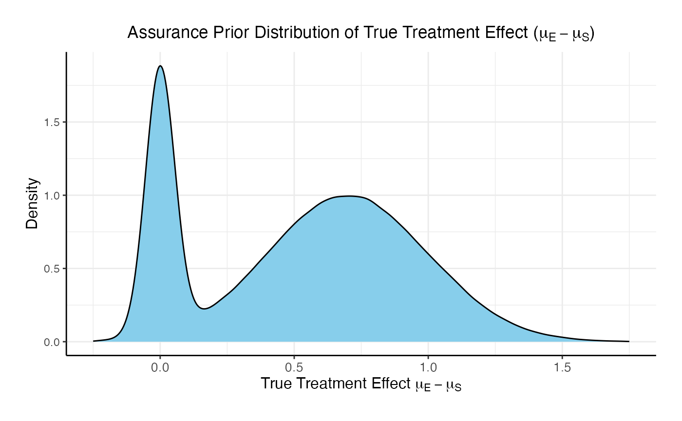
This function simulates patient-level outcomes within a Bayesian assurance framework, using a two-component mixture prior to reflect uncertainty about the true treatment effect. It allows for assessing the probability of trial success (assurance) under uncertainty about the true treatment effect. Information generated from this simulation will be used later for the Analysis Integration Point.

In this example, the true treatment effect ($\mu_E - \mu_S$) is sampled from a mixture of two normal priors:

• 25% weight on $\mathcal{N}(0, 0.05^2)$.
• 75% weight on $\mathcal{N}(0.7, 0.3^2)$.

The control mean is fixed, while the experimental mean is computed as $d\text{MeanCtrl} + \text{treatment effect}$. Each patient’s response is then simulated from a normal distribution corresponding to their assigned treatment group, with standard deviations defined separately for each arm.

Refer to the table below for the definitions and values of the user-defined parameters used in this example.

User parameter	Definition	Value
dWeight1	Weight of prior component 1.	0.25
dWeight2	Weight of prior component 2.	0.75
dMean1	Mean of prior component 1.	0
dMean2	Mean of prior component 2.	0.7
dSD1	Standard deviation of prior component 1.	0.05
dSD2	Standard deviation of prior component 2.	0.3
dMeanCtrl	Mean of control arm (experimental arm will be sampled).	0
dSDCtrl	Standard deviation for control arm.	1.9
dSDExp	Standard deviation for experimental arm.	1.9

Analysis Integration Point

This endpoint is related to this R file: AnalyzeUsingBayesianNormals.R

This function evaluates the posterior probability that the experimental treatment arm is better than the control arm by more than a clinically meaningful threshold, and returns a Go/No-Go decision based on a cutoff ($P_U$). It uses information from the simulation that is generated by the Response element of East Horizon’s simulation, explained above.

For patients receiving treatment $j \in \{\text{S}, \text{E}\}$ (S = standard/control, E = experimental), we assume the outcomes $Y \sim \mathcal{N}(\mu_j, \sigma^2)$, where $\mu_j$ is an unknown mean and $\sigma^2$ is a known, fixed variance.

We assume a priori that:

$$\mu_j \sim \mathcal{N}(\theta_j, \tau_j^2 = 1000^2), \quad j \in \{\text{S}, \text{E}\}$$

After observing $n$ patients on treatment $j$, the posterior distribution of $\mu_j$ becomes:

$$\mu_j \mid \bar{y} \sim \mathcal{N}(\theta_j^*, \tau_j^{2*})$$ where:

$$\theta_j^* = \frac{\frac{\theta_j}{\tau_j^2} + \frac{n \bar{y}}{\sigma^2}}{\frac{1}{\tau_j^2} + \frac{n}{\sigma^2}}, \quad \text{and} \quad \frac{1}{\tau_j^{2*}} = \frac{1}{\tau_j^2} + \frac{n}{\sigma^2}$$

At the conclusion of the study, the posterior probability that the experimental arm exceeds the control arm by more than the minimum acceptable value (MAV) is calculated as:

$$\rho = \Pr(\mu_E > \mu_S + \text{MAV} \mid \text{data})$$

The decision rule is as follows:

• If $\rho > P_U \rightarrow$ Go.
• If $\rho \leq P_U \rightarrow$ No-Go.

Refer to the table below for the definitions and values of the user-defined parameters used in this example.

User parameter	Definition	Value
dPriorMeanCtrl	Prior mean for control arm.	0
dPriorStdDevCtrl	Prior standard deviation for control arm.	1000
dPriorMeanExp	Prior mean for experimental arm.	0
dPriorStdDevExp	Prior standard deviation for experimental arm.	1000
dSigma	Known sampling standard deviation.	1.9
dMAV	Minimum Acceptable Value (clinically meaningful difference).	0.8
dPU	Go threshold (posterior probability cutoff).	0.8

Results

The probability of a Go is 15.3% and the probability of a No-Go is 84.7%.

Example 2 - Group Sequential Design with a Mixture of Normal Distributions

This example follows the same structure and uses the same code as Example 1. However, it introduces an interim analysis (IA) for futility assessment when outcomes are observed for 50% of the enrolled patients. The futility decision is based on the Bayesian predictive probability of a No-Go decision at the end of the trial. Specifically, if the predictive probability suggests that a No-Go is likely at the final analysis, the trial is stopped early for futility. If not, the trial continues to the final analysis (FA), which uses the same R code. The in Analysis element of East Horizon’s simulation is thus customized to handle this case as explained below.

The figure below illustrates where this example fits within the R integration points of Cytel products, accompanied by flowcharts outlining the general steps performed by the R code.

Response (Patient Simulation) Integration Point

This endpoint is related to this R file: SimulatePatientOutcomeNormalAssurance.R

The function for the Response Integration Point is the same as in Example 1. Refer to the table below for the definitions and values of the user-defined parameters used in this example.

User parameter	Definition	Value
dWeight1	Weight of prior component 1.	0.25
dWeight2	Weight of prior component 2.	0.75
dMean1	Mean of prior component 1.	0
dMean2	Mean of prior component 2.	0.7
dSD1	Standard deviation of prior component 1.	0.05
dSD2	Standard deviation of prior component 2.	0.3
dMeanCtrl	Mean of control arm (experimental arm will be sampled).	0
dSDCtrl	Standard deviation for control arm.	1.9
dSDExp	Standard deviation for experimental arm.	1.9

Analysis Integration Point

This endpoint is related to this R file: AnalyzeUsingBayesianNormals.R

The function for the Analysis Integration Point is the same as in Example 1, with the addition of the dPUFutility variable to incorporate the interim analysis. dPUFutility is a user-defined threshold that specifies the minimum predictive probability of a No-Go decision required to stop the trial early for futility at the interim analysis.

Let $X_1$ represent the data available at the interim analysis and $X_2$ the data for patients enrolled thereafter. If the predictive probability of a No-Go decision at the end of the study, given $X_1$, exceeds a pre-specified threshold $PU_{\text{Futility}} = 90\%$, the trial is stopped. Formally, the stopping rule is:

$$\Pr( \text{No-Go at end of study} \mid X_1 ) > PU_{\text{Futility}} = 90\%$$

This can be expressed as:

$$\Pr\left( \left\{ \Pr( \mu_E > \mu_S + MAV \mid X_1, X_2 ) > PU \right\} \Big| X_1 \right) > PU_{\text{Futility}}$$

Refer to the table below for the definitions and values of the user-defined parameters used in this example.

User parameter	Definition	Value
dPriorMeanCtrl	Prior mean for control arm.	0
dPriorStdDevCtrl	Prior standard deviation for control arm.	1000
dPriorMeanExp	Prior mean for experimental arm.	0
dPriorStdDevExp	Prior standard deviation for experimental arm.	1000
dSigma	Known sampling standard deviation.	1.9
dMAV	Minimum Acceptable Value (clinically meaningful difference).	0.8
dPU	Go threshold (posterior probability cutoff).	0.8
dPUFutility	Threshold to stop the trial early for futility.	0.9

Results

The results of the design are as follows:

• The probability of an end of study Go is: 0.1478
• The probability of an end of study No-Go (Stop) is: 0.2656
• The probability of futility at the interim: 0.5866
• The probability of a Go conditional on not stopping at the interim: 0.357523
• The probability of a No-Go conditional on not stopping at the interim: 0.642477

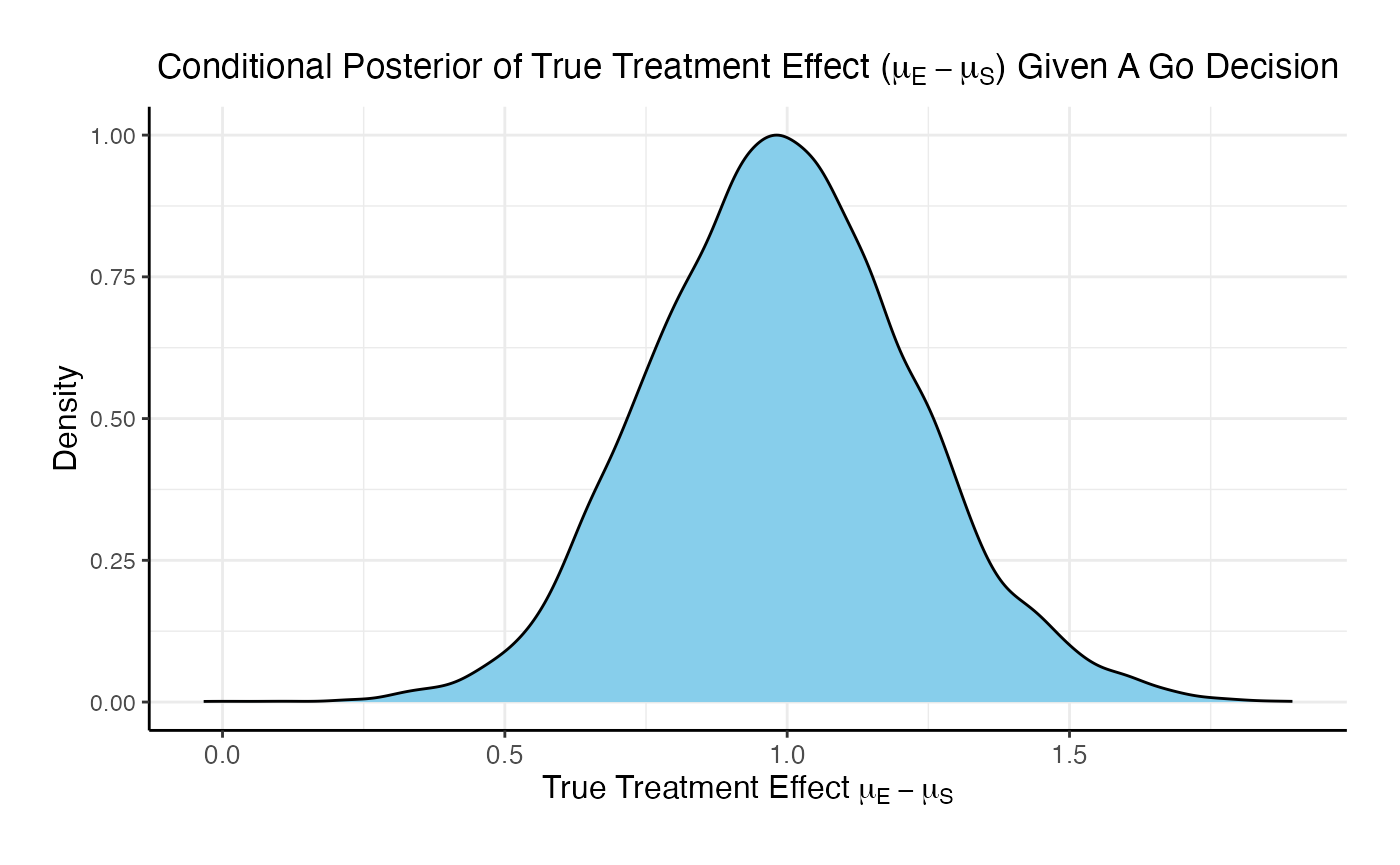
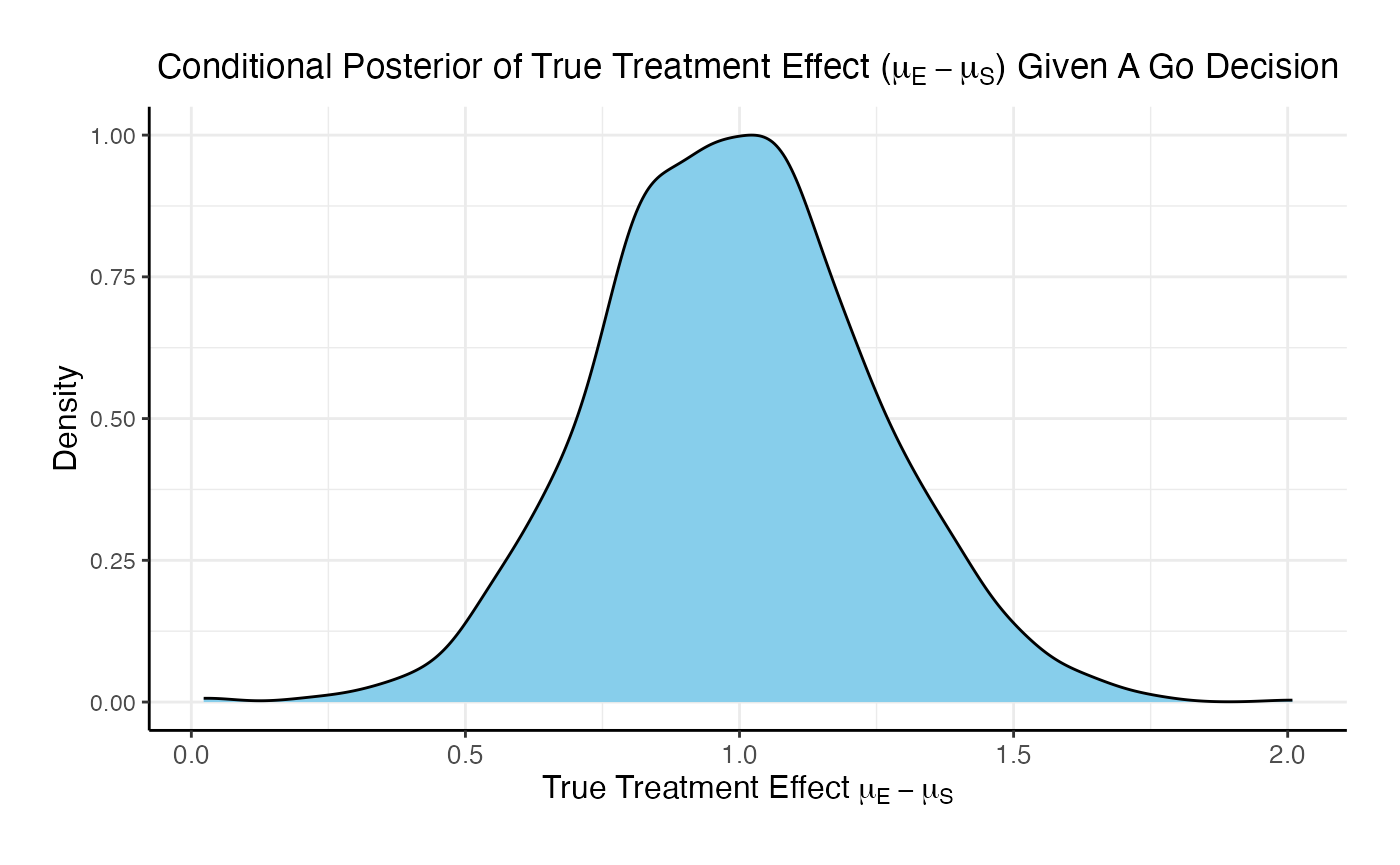
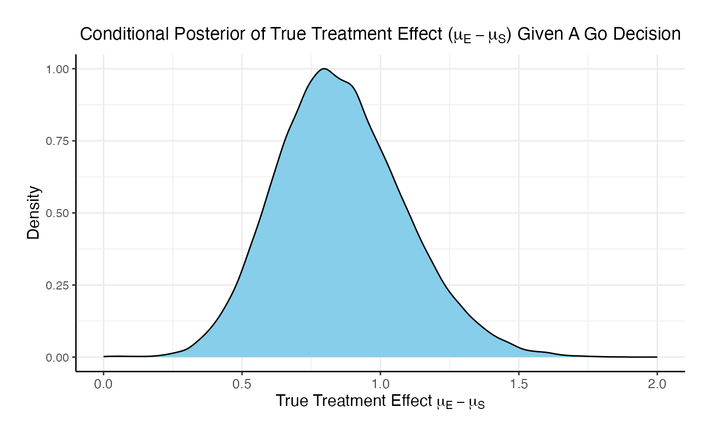
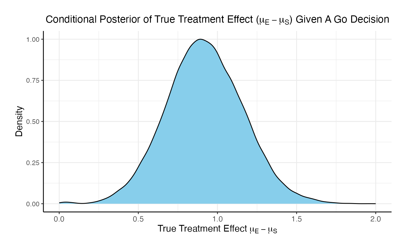
The posterior mean of the true delta, $\mu_E-\mu_S$, given a Go decision is: 0.992

The summary of the true delta given a Go decision is:

##    Min. 1st Qu.  Median    Mean 3rd Qu.    Max. 
##   0.023   0.823   0.990   0.992   1.151   2.009

The scaled posterior distribution of the true delta given a Go decision is:

Example 3 - Fixed Sample Design With a Time-To-Event Outcome

This example considers a two-arm fixed sample design with a time-to-event endpoint, with 300 patients per arm. It demonstrates how to customize the the Response (Patient Simulation) element of East Horizon’s simulation to simulate the true hazard ratio from the prior and then simulate the patient data using the sampled hazard ratio, and the Analysis element of East Horizon’s simulation to perform the analysis using a Cox model.

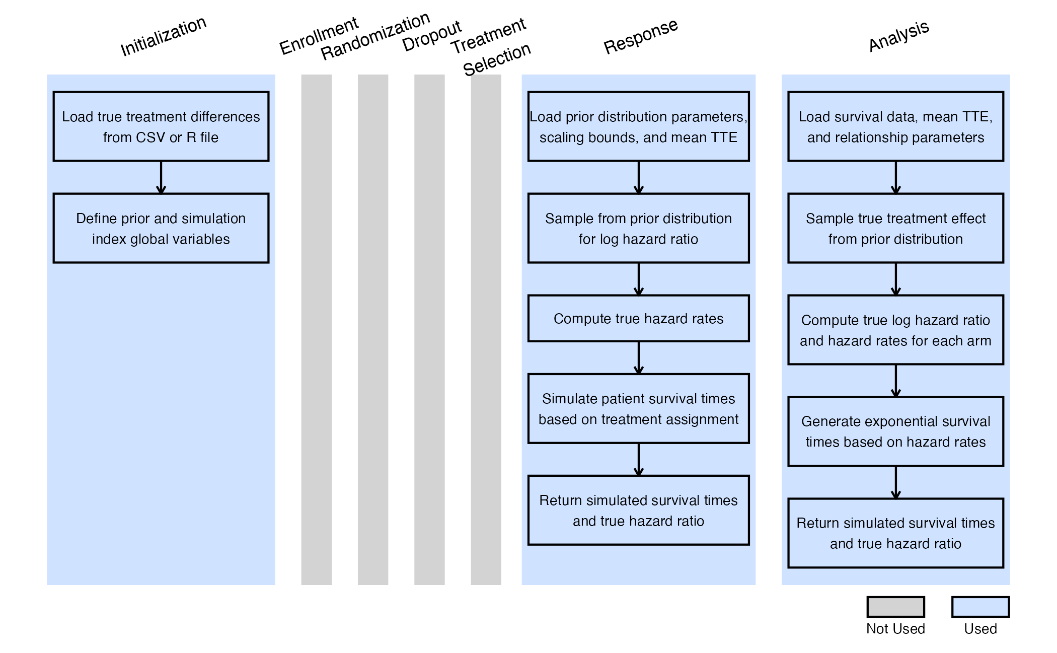
The figure below illustrates where this example fits within the R integration points of Cytel products, accompanied by flowcharts outlining the general steps performed by the R code.

Response (Patient Simulation) Integration Point

This endpoint is related to this R file: SimulatePatientSurvivalAssurance.R

This function simulates patient-level outcomes within a Bayesian assurance framework. Information generated from this simulation will be used later for the Analysis Integration Point. In this example, a bi-modal prior on the $\log(HR)$ is used. The components of the prior are:

• 25% weight on $\mathcal{N}(0, 0.02)$.
• 75% weight on $\mathcal{Beta}(2, 2)$, rescaled between -0.4 and 0.

Refer to the table below for the definitions and values of the user-defined parameters used in this example.

User parameter	Definition	Value
dWeight1	Probability of using the normal prior for log(HR).	0.25
dPriorMean	Mean of the normal prior for log(HR).	0
dPriorSD	Standard deviation of the normal prior for log(HR).	0.02
dAlpha	Alpha parameter of the Beta prior for log(HR).	2
dBeta	Beta parameter of the Beta prior for log(HR).	2
dUpper	Upper bound for scaling the Beta prior.	0
dLower	Lower bound for scaling the Beta prior.	-0.4
dMeanTTEControl	Mean time-to-event for the control group.	12

Analysis Integration Point

This endpoint is related to this R file: AnalyzeSurvivalDataUsingCoxPH.R

A single analysis is conducted once 50% of patients have experienced the event of interest. Using the function in the file, the analysis employs a Cox proportional hazards model, with a hazard ratio (HR) less than 1 indicating a benefit in favor of the experimental arm. It uses information from the simulation that is generated by the Response element of East Horizon’s simulation, explained above. A Go decision is made if the resulting p-value is less than or equal to 0.025. Refer to the table below for the definitions of the user-defined parameters used in this example.

User parameter	Definition
bReturnLogTrueHazard	If True, the function returns the natural logarithm of the true hazard ratio instead of its raw value.
bReturnNAForNoGoTrials	If True and the trial does not meet the Go decision criterion, the function returns NA for the hazard ratio.

Results

The probability of a Go decision is 33% and the probability of a No-Go Decision is is 67%. The posterior distribution of the true $\log( HR )$ given a Go decision is:

Example 4 - Two Consecutive Studies (Normal Outcome) and De-risking

In this section, we explore how to compute assurance and conditional assurance across two sequential studies: a Phase 2 trial followed by a Phase 3 trial, both with a normal endpoint (as in Example 1).

The objective is to understand how conducting a Phase 2 study can reduce the risk associated with the Phase 3 trial. This de-risking is evaluated by comparing two scenarios: (1) the probability of a No-Go decision in Phase 3 if Phase 2 is skipped, and (2) the probability of a No-Go in Phase 3 if a preceding Phase 2 trial is conducted and yields a Go decision. Specifically, we compute the conditional assurance of Phase 3 given success in Phase 2.

Each study of this example customizes the same Integration Points as Example 1, and utilizes the same R code. Please refer to it for more information. The only difference is that we now have two different studies: Phase 3 is conducted only if Phase 2 results in a Go decision.

Phase 2 Study

This study considers a two-arm fixed sample design with normally distributed outcomes $Y$, with 80 patients per treatment arm.

Response (Patient Simulation) Integration Point

This endpoint is related to this R file: SimulatePatientOutcomeNormalAssurance.R

The function for the Response Integration Point of the Phase 2 Study is the same as in Example 1. Refer to the table below for the definitions and values of the user-defined parameters used in this example.

User parameter	Definition	Value
dWeight1	Weight of prior component 1.	0.25
dWeight2	Weight of prior component 2.	0.75
dMean1	Mean of prior component 1.	0
dMean2	Mean of prior component 2.	0.7
dSD1	Standard deviation of prior component 1.	0.05
dSD2	Standard deviation of prior component 2.	0.3
dMeanCtrl	Mean of control arm (experimental arm will be sampled).	0
dSDCtrl	Standard deviation for control arm.	1.9
dSDExp	Standard deviation for experimental arm.	1.9

Analysis Integration Point

This endpoint is related to this R file: AnalyzeUsingBayesianNormals.R

The function for the Analysis Integration Point of the Phase 2 Study is the same as in Example 1.

For this study, the MAV is set to 0.6 and $P_U$ to 0.8. Refer to the table below for all the definitions and values of the user-defined parameters used in this example.

User parameter	Definition	Value
dPriorMeanCtrl	Prior mean for control arm.	0
dPriorStdDevCtrl	Prior standard deviation for control arm.	1000
dPriorMeanExp	Prior mean for experimental arm.	0
dPriorStdDevExp	Prior standard deviation for experimental arm.	1000
dSigma	Known sampling standard deviation.	1.9
dMAV	Minimum Acceptable Value (clinically meaningful difference).	0.6
dPU	Go threshold (posterior probability cutoff).	0.8

Phase 3 Study

This study considers a two-arm fixed sample design with normally distributed outcomes $Y$, with 200 patients per treatment arm.

Response (Patient Simulation) Integration Point

This endpoint is related to this R file: SimulatePatientOutcomeNormalAssurance.R

The function for the Response Integration Point of the Phase 2 Study is the same as in Example 1. Refer to the table below for the definitions and values of the user-defined parameters used in this example.

User parameter	Definition	Value
dWeight1	Weight of prior component 1.	0.25
dWeight2	Weight of prior component 2.	0.75
dMean1	Mean of prior component 1.	0
dMean2	Mean of prior component 2.	0.7
dSD1	Standard deviation of prior component 1.	0.05
dSD2	Standard deviation of prior component 2.	0.3
dMeanCtrl	Mean of control arm (experimental arm will be sampled).	0
dSDCtrl	Standard deviation for control arm.	1.9
dSDExp	Standard deviation for experimental arm.	1.9

Analysis Integration Point

This endpoint is related to this R file: AnalyzeUsingBayesianNormals.R

The function for the Analysis Integration Point of the Phase 2 Study is the same as in Example 1.

For this study, the MAV is set to 0.6 and $P_U$ to 0.5. This design is equivalent to a t-test because the critical value would be 0.6 and having a posterior probability greater than 0.5 would indicate that the estimated treatment difference is above the critical value.

Refer to the table below for all the definitions and values of the user-defined parameters used in this example.

User parameter	Definition	Value
dPriorMeanCtrl	Prior mean for control arm.	0
dPriorStdDevCtrl	Prior standard deviation for control arm.	1000
dPriorMeanExp	Prior mean for experimental arm.	0
dPriorStdDevExp	Prior standard deviation for experimental arm.	1000
dSigma	Known sampling standard deviation.	1.9
dMAV	Minimum Acceptable Value (clinically meaningful difference).	0.6
dPU	Go threshold (posterior probability cutoff).	0.5

Results

For the phase 2 study independently, the probability of a Go is 26.7% and the probability of a No-Go is 73.3%.

For the phase 3 study independently, the probability of a Go is 46% and the probability of a No-Go is 54%.

If the two studies are run sequentially, conducting Phase 3 only if Phase 2 results in a Go decision, the probability of a Go in Phase 3 is 84.8% and the probability of a No-Go is 15.2%.

Comparing the option of running only a Phase 3 versus a Phase 2 followed by a Phase 3 if Phase 2 is successful, the probability of Go in phase 3 increases from 46% to 84.8% and the probability of a No-Go in Phase 3 decreases from 54% to 15.2%.

Example 5 - Two Consecutive Studies (Normal and Time-To-Event outcomes) and De-risking

Similarly to Example 4, in this section we explore how to compute assurance and conditional assurance across two sequential studies: a Phase 2 trial with a normal endpoint followed by a Phase 3 trial with a time-to-event endpoint.

As before, Phase 3 is conducted only if Phase 2 results in a Go decision. The Phase 2 study of this example customizes the same Integration Points as Example 1, and utilizes the same R code. Please refer to it for more information. However, the Phase 3 study utilizes new Integration points and R code, as described below.

Phase 2 Study

This study considers a two-arm fixed sample design with normally distributed outcomes $Y$, with 80 patients per treatment arm.

Response (Patient Simulation) Integration Point

This endpoint is related to this R file: SimulatePatientOutcomeNormalAssurance.R

The function for the Response Integration Point of the Phase 2 Study is the same as in Example 1. Refer to the table below for the definitions and values of the user-defined parameters used in this example.

User parameter	Definition	Value
dWeight1	Weight of prior component 1.	0.25
dWeight2	Weight of prior component 2.	0.75
dMean1	Mean of prior component 1.	0
dMean2	Mean of prior component 2.	0.7
dSD1	Standard deviation of prior component 1.	0.05
dSD2	Standard deviation of prior component 2.	0.3
dMeanCtrl	Mean of control arm (experimental arm will be sampled).	0
dSDCtrl	Standard deviation for control arm.	1.9
dSDExp	Standard deviation for experimental arm.	1.9

Analysis Integration Point

This endpoint is related to this R file: AnalyzeUsingBayesianNormals.R

The function for the Analysis Integration Point of the Phase 2 Study is the same as in Example 1.

For this study, the MAV is set to 0.6 and $P_U$ to 0.8. Refer to the table below for all the definitions and values of the user-defined parameters used in this example.

User parameter	Definition	Value
dPriorMeanCtrl	Prior mean for control arm.	0
dPriorStdDevCtrl	Prior standard deviation for control arm.	1000
dPriorMeanExp	Prior mean for experimental arm.	0
dPriorStdDevExp	Prior standard deviation for experimental arm.	1000
dSigma	Known sampling standard deviation.	1.9
dMAV	Minimum Acceptable Value (clinically meaningful difference).	0.6
dPU	Go threshold (posterior probability cutoff).	0.8

Phase 3 Study

This study considers a two-arm fixed sample design with a time-to-event endpoint, with 300 patients per arm.

The figure below illustrates where the integration points used in this study fit within the R integration points of Cytel products, accompanied by flowcharts outlining the general steps performed by the R code.

Initialize Integration Point

This endpoint is related to this R file: ReadInPrior.R

During the Phase 2 simulation, the true treatment difference was sampled from the prior distribution and we manually saved it to an output CSV file.

Both conditional and unconditional Phase 3 simulations use an R initialization function to load this output and extract the true treatment differences. These values are then converted to the log of the true hazard ratio (HR) using the linear link function shown in the Response section. Note that while unconditional assurance could be calculated by sampling directly from the Phase 2 prior, reading the saved values ensures a consistent comparison between conditional and unconditional assurance. This approach provides a more accurate assessment of the benefit of conducting a Phase 2 trial before Phase 3.

If used with East, the ReadExample5Phase2Output function is used to load the true treatment differences from a CSV file. You can update the R code to specify your correct file path. In East Horizon, which does not support file uploads, use the ReadExample5Phase2OutputSolara function instead. There, the treatment differences are pasted directly into an R vector.

In the R code, note that the <<- operator is used to define two global variables:

• vPrior: a vector containing the true treatment differences.
• nSimIndex: an index tracking the current replication being executed during the Phase 3 simulation.

Both variables are used in the Response Integration Point R function. The nSimIndex value is updated with each simulation iteration.

This function relies on the user-defined parameter bConditionalOnGo. When set to 1, only the true treatment differences that led to a Go decision in Phase 2 are used to calculate conditional assurance. Note that the number of Phase 3 replications used in simulating for conditional assurance must be no greater than the number of successful Phase 2 simulations. When bConditionalOnGo is set to 0, all sampled treatment differences from Phase 2 are used to compute unconditional assurance. Refer to the table below for the definitions of the user-defined parameters used in this example.

User parameter	Definition
bConditionalOnGo	If True, uses only Phase 2 results that led to a Go decision. Otherwise, uses all results.

Response (Patient Simulation) Integration Point

This endpoint is related to this R file: SimulatePatientSurvivalAssuranceUsingPh2Prior.R

This function simulates patient-level outcomes within a Bayesian assurance framework. The relationship between the continuous endpoint in Phase 2 and the time-to-event endpoint in Phase 3 is modeled using a linear function:

$$\log(\text{True HR})_{\text{Phase 3}} = 0.1 - 0.4 \times (\text{True Treatment Difference})_{\text{Phase 2}}$$

Note that this relationship is defined in terms of the true treatment effects. Since Phase 2 informs the prior on the true treatment difference and a direct link is established between the true difference and the true hazard ratio, there is no need to specify a separate prior for the true HR as done in Example 3.

Refer to the table below for the definitions and values of the user-defined parameters used in this example.

User parameter	Definition	Value
dMeanTTEControl	Mean time-to-event for the control group.	12
dIntercept	Intercept for the linear relationship between true treatment difference and log(HR).	0.1
dSlope	Slope for the linear relationship between true treatment difference and log(HR).	-0.4

Analysis Integration Point

This endpoint is related to this R file: AnalyzeSurvivalDataUsingCoxPH.R

Similarly to Example 3, a single analysis is conducted once 50% of patients have experienced the event of interest. Using the function in the file, the analysis employs a Cox proportional hazards model, with a hazard ratio (HR) less than 1 indicating a benefit in favor of the experimental arm. A Go decision is made if the resulting p-value is less than or equal to 0.025.

Refer to the table below for the definitions of the user-defined parameters used in this example.

User parameter	Definition
bReturnLogTrueHazard	If True, the function returns the natural logarithm of the true hazard ratio instead of its raw value.
bReturnNAForNoGoTrials	If True and the trial does not meet the Go decision criterion, the function returns NA for the hazard ratio.

Results

For the phase 2 study independently, the probability of a Go is 26.7% and the probability of a No-Go is 73.3%.

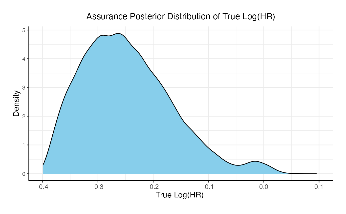
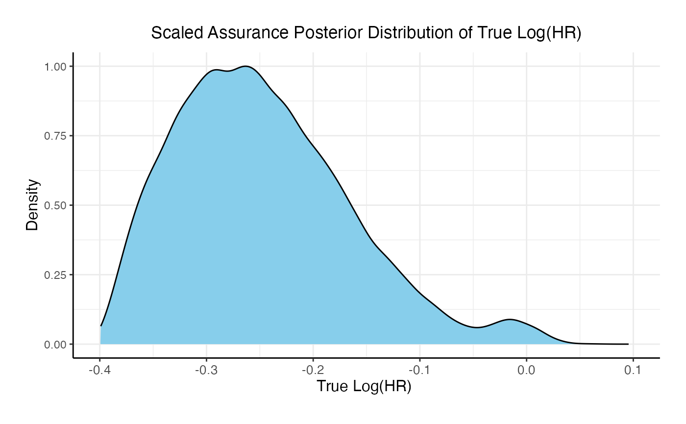
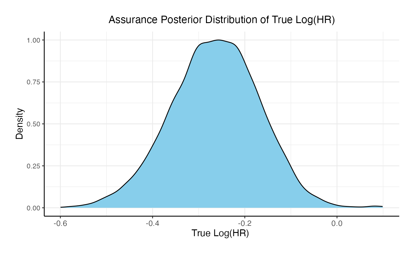
For the phase 3 study independently, the unconditional probability of a Go decision is 29% and the unconditional probability of a No-Go Decision is 71%. The 95% posterior credible for the Log( True HR ) is (-$\infty$, 0.12 ). The posterior distribution of the true Log( HR ) given a Go decision is:

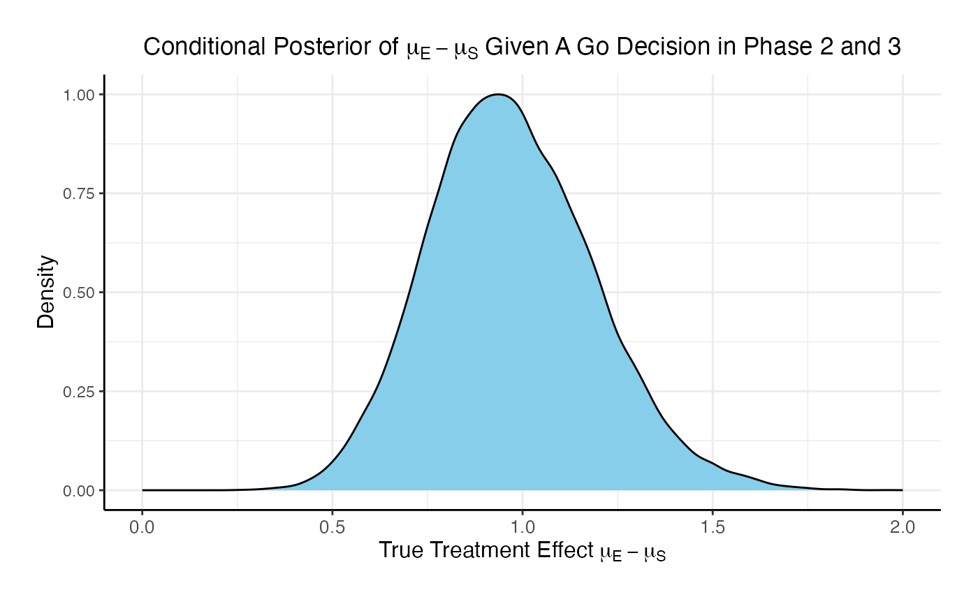
If the two studies are run sequentially, conducting Phase 3 only if Phase 2 results in a Go decision, the probability of a Go decision is 60% and the unconditional probability of a No-Go Decision is 40%. The 95% posterior credible for the Log( True HR ) is (-0.46, -0.08). The posterior distribution of the true Log( HR ) given a Phase 3 Go decision is:

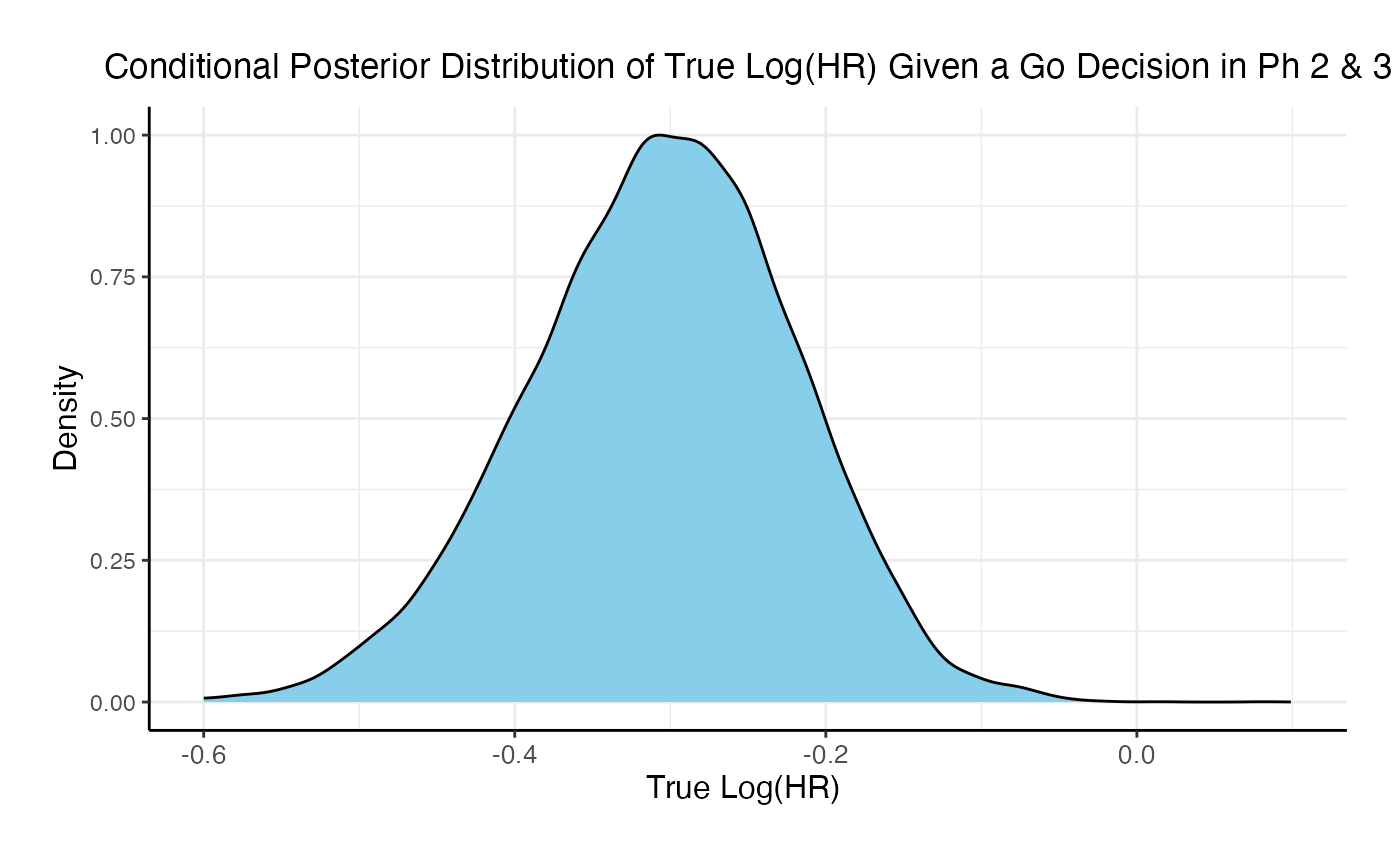
Comparing the option of running only a Phase 3 versus a Phase 2 followed by a Phase 3 if Phase 2 is successful, the probability of Go in phase 3 increases from 29% to 60% and the probability of a No-Go in Phase 3 decreases from 71% to 40%.