2-Arm, Normal Outcome - Analysis

Shubham Lahoti and J. Kyle Wathen

June 04, 2025

These examples are related to the Integration Point: Analysis - Continuous Outcome. Click here for more information about this integration point.

Introduction

The following examples illustrate how to integrate new analysis capabilities into East Horizon or East using R functions in the context of a two-arm trial. In each example, the trial design includes a standard-of-care control arm and an experimental treatment arm, with patient outcomes assumed to follow a normal distribution. The design includes two interim analyses (IA) and one final analysis (FA). At each IA, an analysis is conducted which may lead to early stopping for efficacy or futility, depending on the predefined design criteria.

Once CyneRgy is installed, you can load this example in RStudio with the following commands:

CyneRgy::RunExample( "2ArmNormalOutcomeAnalysis" )

Running the command above will load the RStudio project in RStudio.

East Workbook: 2ArmNormalOutcomeAnalysis.cywx

RStudio Project File: 2ArmNormalOutcomeAnalysis.Rproj

In the R directory of this example you will find the following R files:

1. AnalyzeUsingEastManualFormulaNormal.R - Contains a function named AnalyzeUsingEastManualFormulaNormal to demonstrate the R code necessary for Example 1 as described below.

2. AnalyzeUsingTTestNormal.R - Contains a function named AnalyzeUsingTTestNormal to demonstrate the R code necessary for Example 2 as described below.

3. AnalyzeUsingMeanLimitsOfCI.R - Contains a function named AnalyzeUsingMeanLimitsOfCI to demonstrate the R code necessary for Example 3 as described below.

Example 1 - Using Formulas Q.3.3 from the East manual

This example is related to this R file: AnalyzeUsingEastManualFormulaNormal.R

In this example, the analysis is customized by replacing the default method with a user-defined calculation based on formulas of the Appendix Q.3.3 - Parallel Design: Difference of Means from the East manual.

Estimate of the pooled standard deviation:

$$\hat\sigma^{2} = \sqrt{ \frac{(n_t - 1) \cdot \sigma_t^2 + (n_c - 1) \cdot \sigma_c^2} {n - 2} }$$

Where:

• $n_t$ and $n_c$ are the number of patients in the treatment and control groups, respectively.
• $\hat\sigma_t$ and $\hat\sigma_e$ are the standard deviations of responses in the treatment and control groups, respectively.
• $n = n_t + n_c$ is the total number of patients.

Test Statistic:

$$Z = \frac{\hat{\mu}_t - \hat{\mu}_c} { \sqrt{\hat\sigma^{2} \cdot (\frac{1}{n_c} + \frac{1}{n_t})}}$$

Where:

• $\hat{\mu}_t$ and $\hat{\mu}_e$ are the means of responses in the treatment and control groups, respectively.
• $\hat\sigma^{2}$ is the estimate of the pooled standard deviation.
• $n_t$ and $n_c$ are the numbers of patients in the treatment and control groups, respectively.

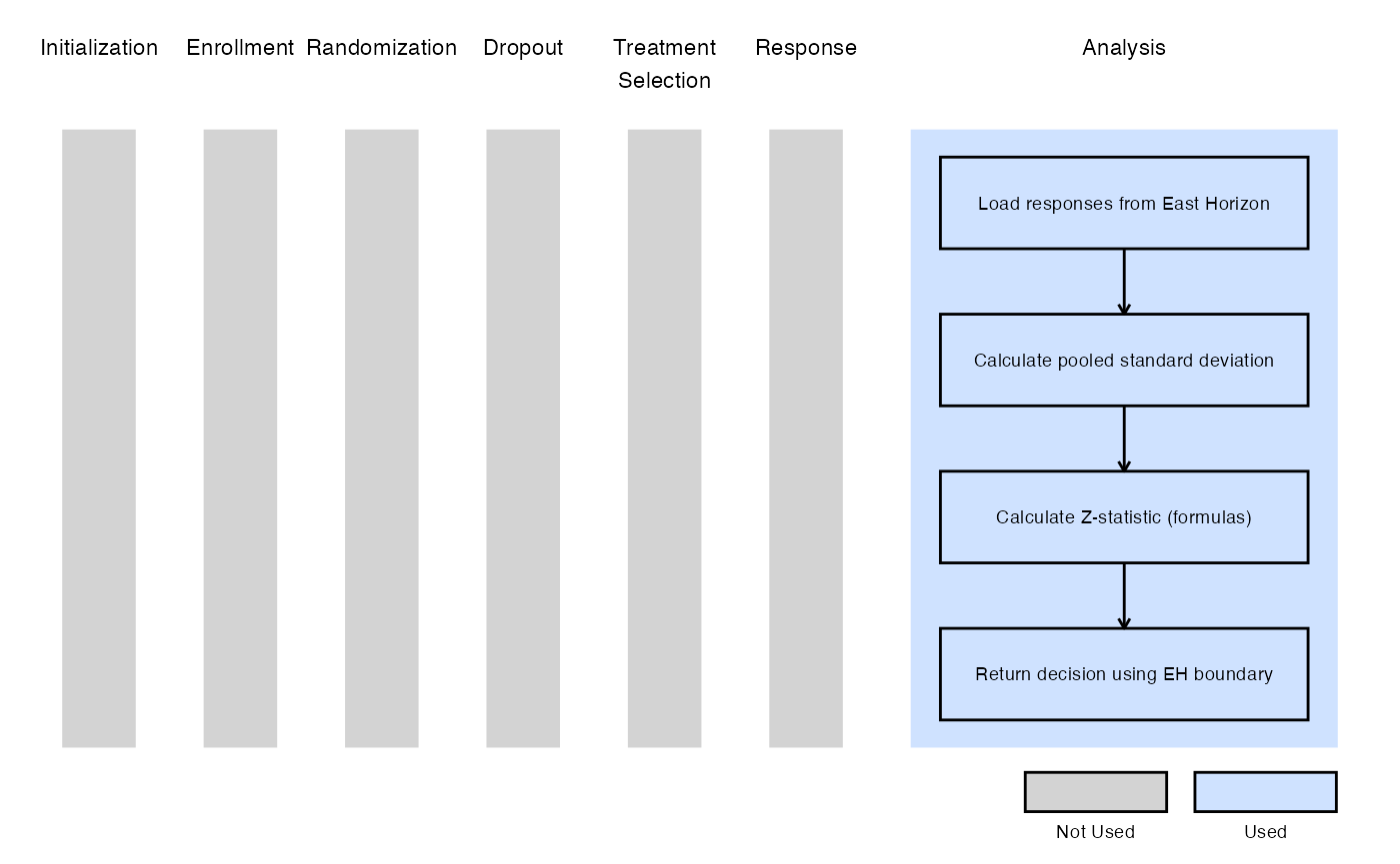
The objective is to demonstrate a straightforward way to modify both the analysis and decision-making process. The computed test statistic is compared to the efficacy boundary provided by East Horizon or East as input. This example does not include a futility rule and does not use any user-defined parameters.

The figure below illustrates where this example fits within the R integration points of Cytel products, accompanied by a flowchart outlining the general steps performed by the R code.

Example 2 - Using the t.test() Function in R

This example is related to this R file: AnalyzeUsingTTestNormal.R

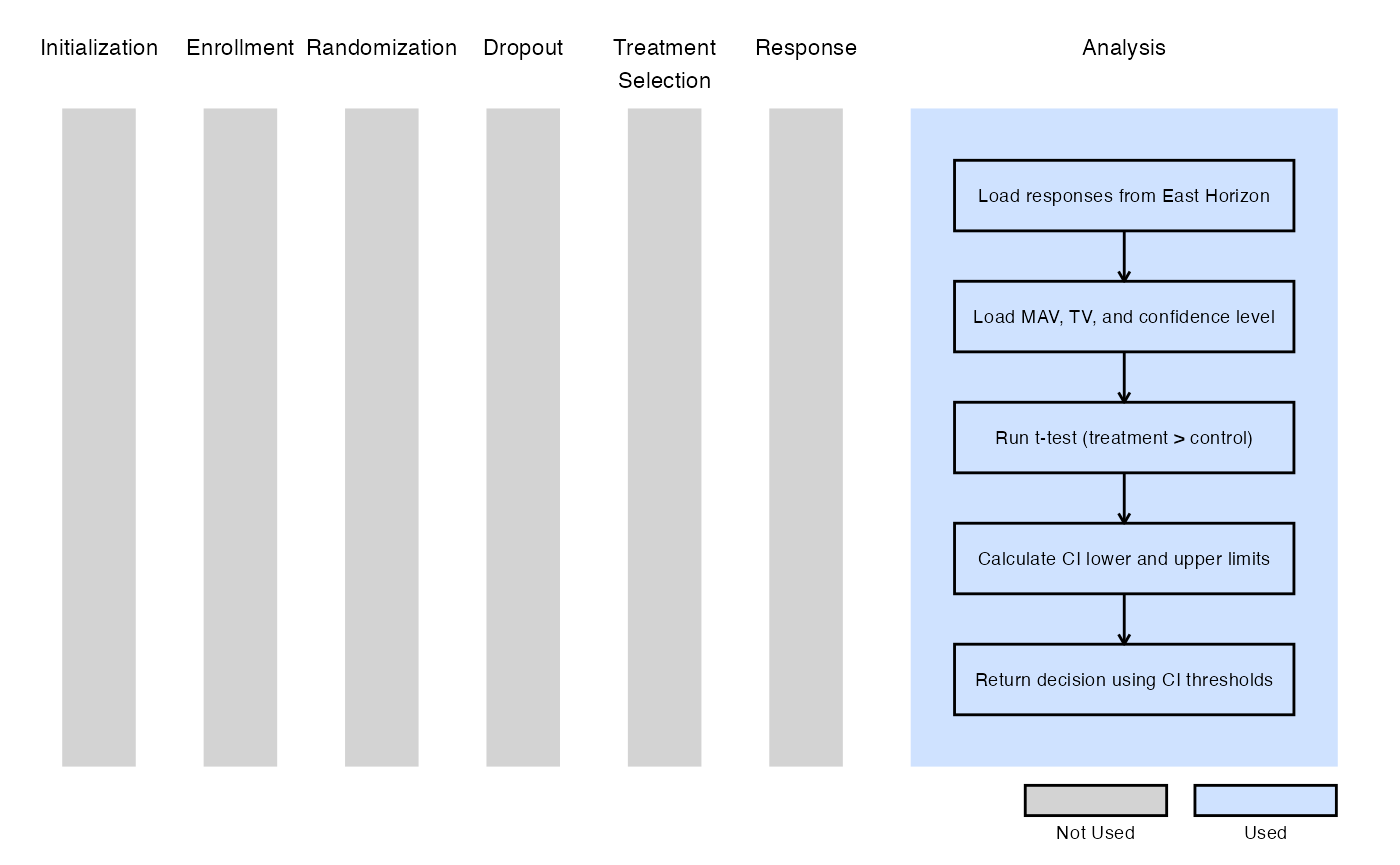
This example utilizes the base R t.test() function to perform the interim and final analyses. The resulting t-statistic is compared against the efficacy boundary provided by East Horizon or East. Like Example 1, this example does not include a futility rule and does not use any user-defined parameters.

The figure below illustrates where this example fits within the R integration points of Cytel products, accompanied by a flowchart outlining the general steps performed by the R code.

Example 3 - Utilization of Confidence Interval Limits for Go/No-Go Decision-Making

This example is related to this R file: AnalyzeUsingMeanLimitsOfCI.R

In many Phase II trials, Go/No-Go decisions are made based on whether a treatment shows sufficient promise to justify further development. These decisions are often guided by two key thresholds:

• Minimum Acceptable Value (MAV): The smallest treatment effect considered meaningful.
• Target Value (TV): A highly desirable treatment effect based on clinical or strategic considerations.

This example demonstrates how to approximate probabilistic decision-making using frequentist confidence intervals (CIs), ignoring the boundaries provided by East Horizon or East in favor of a CI-based logic. We use the function t.test() from base R to analyze the data and compute the desired confidence intervals. If the treatment difference is likely to exceed the MAV, a Go decision is made. If not, and it is unlikely to exceed the TV, a No-Go decision is made. Specifically:

At Interim Analysis

• Let LL and UL be the lower and upper limits of the confidence interval for the treatment effect.
• If $LL > \text{MAV} \rightarrow \text{Go}$
• If $UL < \text{TV} \rightarrow \text{No-Go}$
• Otherwise $\rightarrow$ Continue to the next analysis

At Final Analysis

• If $LL > \text{MAV} \rightarrow \text{Go}$
• Otherwise $\rightarrow$ No-Go

In this example, the team has resources for 100 patients and is comparing two fixed designs and one group sequential design with a single interim analysis. Refer to the table below for the definitions of the user-defined parameters used in this example.

User parameter	Definition
dMAV	Minimum Acceptable Value: the smallest treatment effect considered clinically meaningful to warrant further development.
dTV	Target Value: the desired treatment effect that would represent a strong clinical benefit or strategic advantage.
dConfLevel	Confidence Level: the level of confidence used to construct the confidence interval for Go/No-Go decision-making (e.g., 0.80 for an 80% CI).

Note: In this example, the boundary information that is computed in East Horizon or East is ignored. User-defined parameters and the function t.test() from base R are used to analyze the data and compute the desired confidence intervals.

The figure below illustrates where this example fits within the R integration points of Cytel products, accompanied by a flowchart outlining the general steps performed by the R code.

Option 1 - Fixed Design (80% CI)

The decisions are made as follows:

• Go: If there is at least a 90% probability that the treatment effect exceeds MAV = 0.1 (approximated by lower bound of 80% CI > MAV).
• No-Go: If a Go decision is not made, and there is less than a 10% probability that the effect exceeds TV = 0.3 (approximated by upper bound of 80% CI < TV).

This framework can be approximated using frequentist logic by applying the decision rules to an 80% confidence interval assuming to range from the 10th to the 90th percentile.

Refer to the table below for the values of the user-defined parameters used in this option.

User parameter	Value
dMAV	0.1
dTV	0.3
dConfLevel	0.8

Option 2 - Fixed Design (70% CI)

The decisions are made as follows:

• Go: If there is at least an 85% probability that the treatment effect exceeds MAV = 0.1 (approximated by lower bound of 70% CI > MAV).
• No-Go: If a Go decision is not made, and there is less than a 15% probability that the effect exceeds TV = 0.3 (approximated by upper bound of 70% CI < TV).

This framework can be approximated using frequentist logic by applying the decision rules to an 80% confidence interval assuming to range from the 15th to the 85th percentile.

Refer to the table below for the values of the user-defined parameters used in this option.

User parameter	Value
dMAV	0.1
dTV	0.3
dConfLevel	0.7

Option 3 - Group Sequential Design

In this option, an interim analysis at 50 patients is included with an option to stop for early Go or No-Go decision.

The decisions are made as follows:

• Go (or continue to the next analysis if IA): If there is at least an 92.5% probability that the treatment effect exceeds MAV = 0.1 (approximated by lower bound of 85% CI > MAV).
• No-Go (or stop for futility if IA): If a Go decision is not made, and there is less than a 7.5% probability that the effect exceeds TV = 0.3 (approximated by upper bound of 85% CI < TV).

This framework can be approximated using frequentist logic by applying the decision rules to an 85% confidence interval assuming to range from the 7.5 to the 92.5th percentile.

Refer to the table below for the values of the user-defined parameters used in this option.

User parameter	Value
dMAV	0.1
dTV	0.3
dConfLevel	0.85