2 Arm, Time-To-Event Outcome - Patient Simulation • CyneRgy

These examples are related to the Integration Point: Response - Time-to-Event Outcome. Click here for more information about this integration point.

Introduction

The following examples illustrate how to integrate new patient outcome simulation (response) capabilities into East Horizon or East using R functions in the context of a two-arm trial. In each example, the trial design includes a standard-of-care control arm and an experimental treatment arm, with patient outcomes modeled as time-to-event data.

Once CyneRgy is installed, you can load this example in RStudio with the following commands:

CyneRgy::RunExample( "2ArmTimeToEventOutcomePatientSimulation" )

Running the command above will load the RStudio project in RStudio.

East Workbook: 2ArmTimeToEventOutcomePatientSimulation.cywx

RStudio Project File: 2ArmTimeToEventOutcomePatientSimulation.Rproj

In the R directory of this example you will find the following R files:

SimulatePatientSurvivalWeibull.R - This file provides an example R function to simulate patient time-to-event data from a Weibull distribution.
SimulatePatientSurvivalMixtureExponentials.R - This file provides an example R function to simulate patient data from a mixture of exponential distributions. The mixture is based on having any number of patient groups in the study where each group has a different exponential distribution for simulating the time-to-event from.

Example 1 - Simulation of Patient Time-To-Event Data from a Weibull Distribution

This example is related to this R file: SimulatePatientSurvivalWeibull.R

In this example, the R function SimulatePatientSurvivalWeibull is provided to simulate patient data with hazards and hazard ratios that change over time, allowing for an exploration of their impact on expected study power. Refer to the table below for the definitions of the user-defined parameters used in this example.

User parameter	Definition
dShapeCtrl	Shape parameter of the Weibull distribution for the control arm.
dShapeExp	Shape parameter of the Weibull distribution for the experimental arm.
dScaleCtrl	Scale parameter of the Weibull distribution for the control arm.
dScaleExp	Scale parameter of the Weibull distribution for the experimental arm.

The figure below illustrates where this example fits within the R integration points of Cytel products, accompanied by a flowchart outlining the general steps performed by the R code.

Example 1.1 – Constant Hazards

Assume that the difference in risk of death for patients in the control arm compared to the risk of death for patients in the experimental arm remains the same over time. The time to death or progression of patients is simulated from a Weibull distribution with the shape and scale for each arm provided in East Horizon or East and sent to R. Refer to the table below for the values of the user-defined parameters used in this example.

User parameter	Value
dShapeCtrl	1.0
dShapeExp	1.0
dScaleCtrl	17.31
dScaleExp	23.08

The scale parameters are calculated based on the median survival time for each arm. This example demonstrates that using the R function with these parameters produces the same results as simulating the data directly in East Horizon or East without an R function.

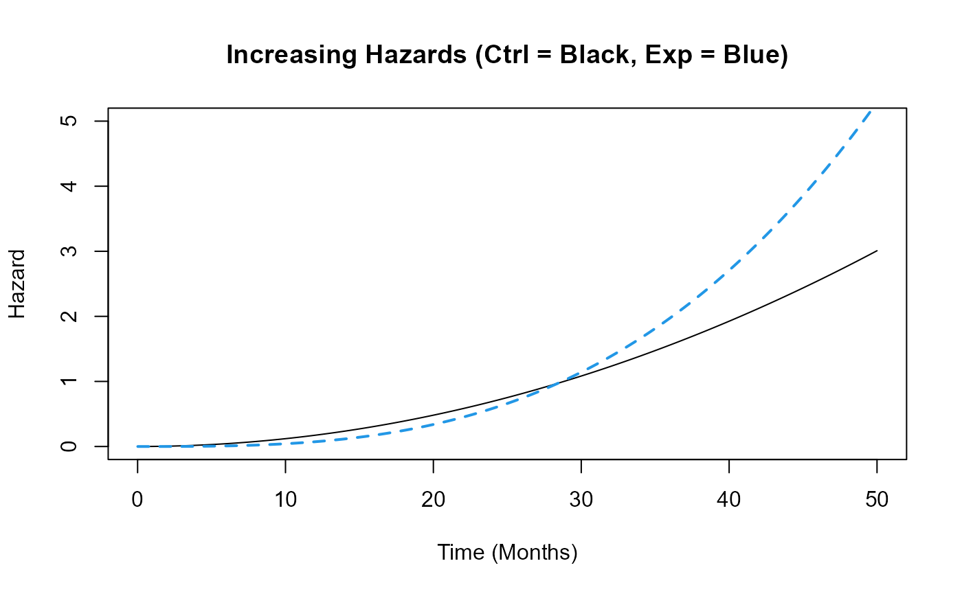
Example 1.2 – Increasing Hazards

This function assumes that the hazard of death or disease progression increases over time in both arms, but at different rates: the control arm’s hazard increases more slowly than that of the experimental arm. The time to death or progression is simulated using a Weibull distribution, with shape and scale parameters specified for each arm in East Horizon or East and then sent to R. Refer to the table below for the values of the user-defined parameters used in this example.

User parameter	Value
dShapeCtrl	3.0
dShapeExp	4.0
dScaleCtrl	13.56
dScaleExp	17.54

This example demonstrates how an R function can be used to simulate data in a way that differs from East Horizon’s or East’s default simulation approach.

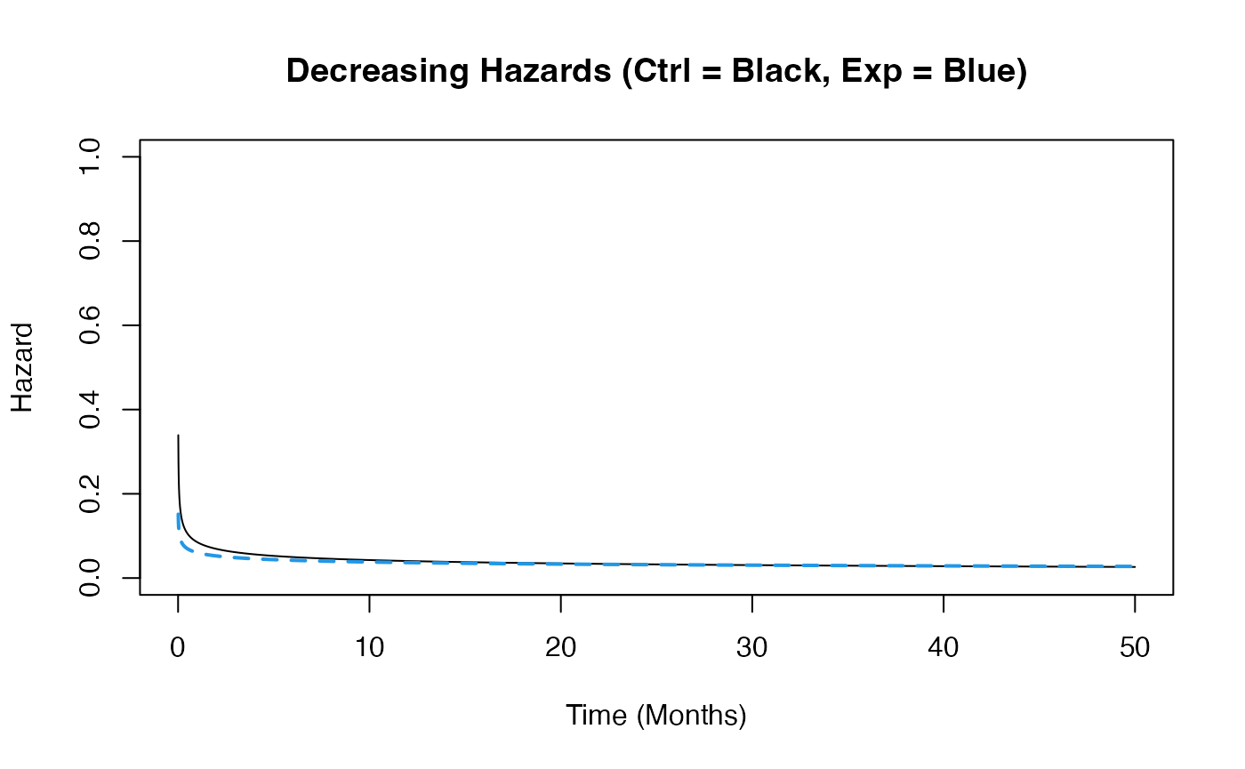
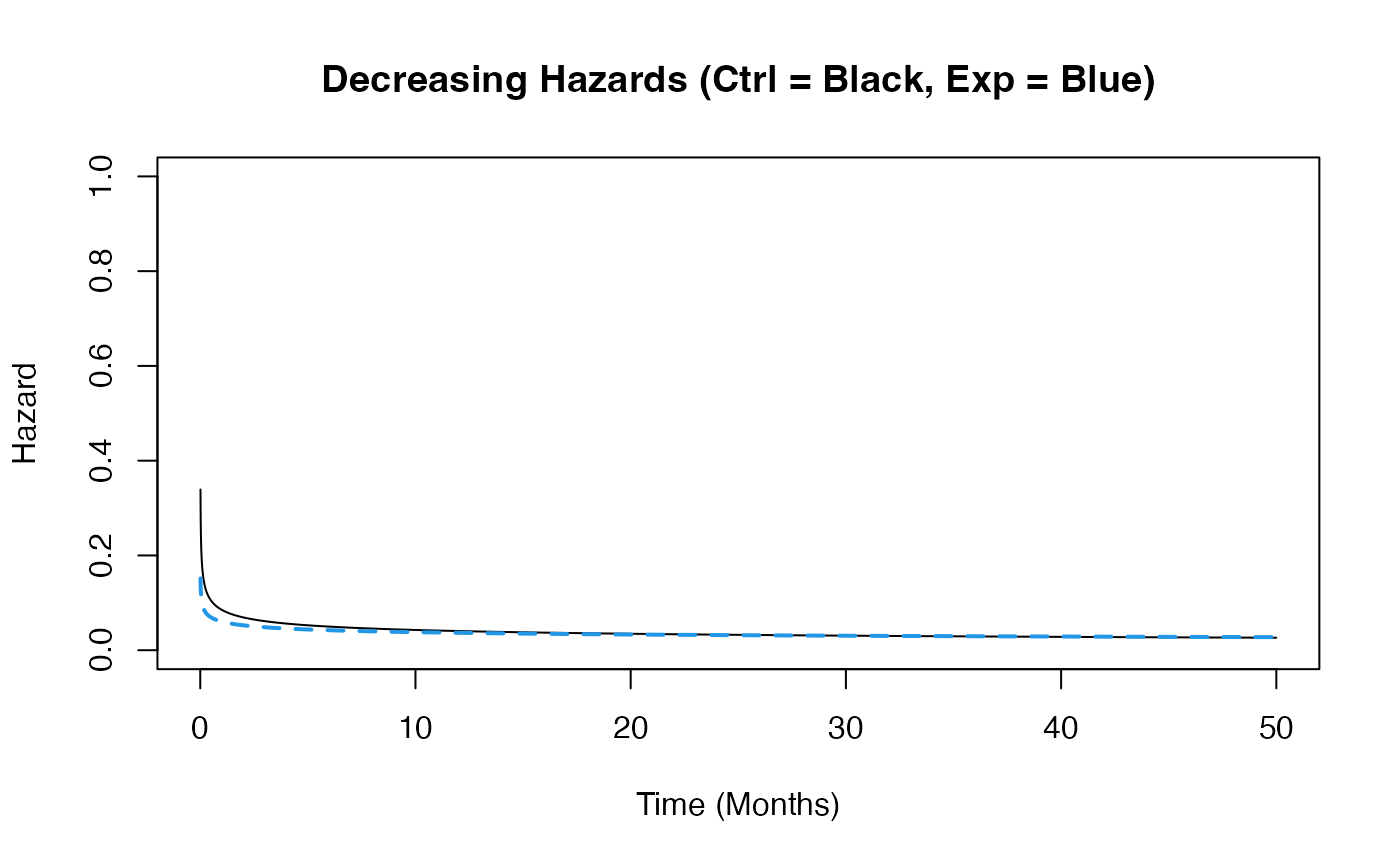
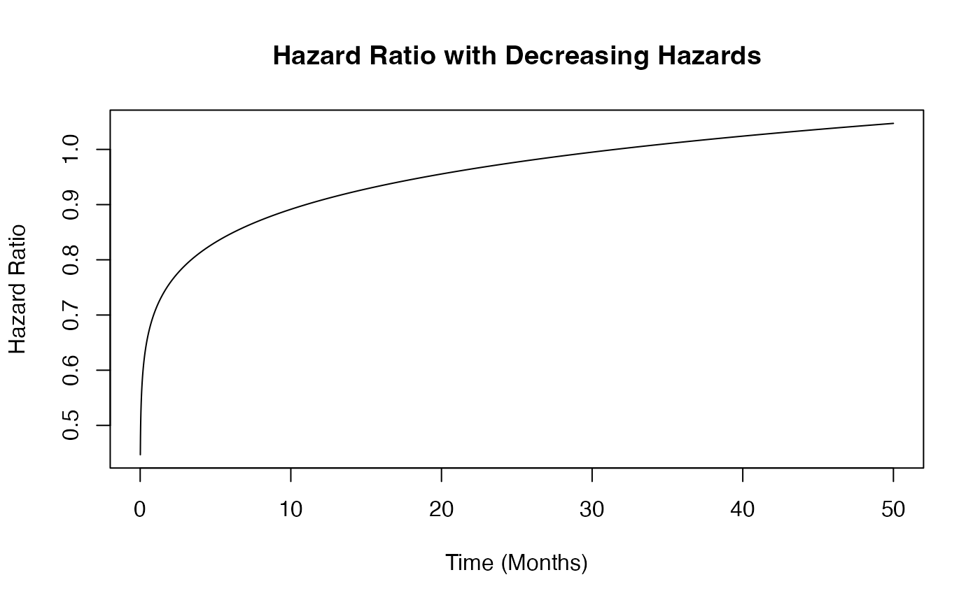
Example 1.3 – Decreasing Hazards

This example is similar to the previous one, but here the function assumes that hazards decrease over time in both arms. However, the control arm’s hazard decreases at a slower rate than that of the experimental arm. The time to death or progression is simulated using a Weibull distribution, with shape and scale parameters specified for each arm in East Horizon or East and then sent to R. Refer to the table below for the values of the user-defined parameters used in this example.

User parameter	Value
dShapeCtrl	0.7
dShapeExp	0.8
dScaleCtrl	20.26
dScaleExp	25.30

This example demonstrates how an R function can be used to simulate data differently from East Horizon’s or East’s default simulation approach.

Example 2 - Simulation of Patient Time-To-Event Data from a Mixture of Distributions

This example is related to this R file: SimulatePatientSurvivalMixtureExponentials.R

This example simulates patient data using a mixture of exponential distributions, allowing for multiple patient subgroups within the study. Each subgroup follows a distinct exponential distribution for modeling TTE, capturing variability in patient outcomes. Refer to the table below for the definitions of the user-defined parameters used in this example.

User parameter	Definition
QtyOfSubgroups	Number of patient subgroups.
ProbSubgroup1	Probability a patient is in subgroup 1.
MedianTTECtrlSubgroup1	Median time-to-event for a patient in subgroup 1 that receives control treatment.
MedianTTEExpSubgroup1	Median time-to-event for a patient in subgroup 1 that receives experimental treatment.
ProbSubgroup2	Probability a patient is in subgroup 2.
MedianTTECtrlSubgroup2	Median time-to-event for a patient in subgroup 2 that receives control treatment.
MedianTTEExpSubgroup2	Median time-to-event for a patient in subgroup 2 that receives experimental treatment.
…	Probabilities and median time-to-event for additional subgroups follow the same format, incrementing the subgroup number (e.g., ProbSubgroup3, MedianTTECtrlSubgroup3, MedianTTEExpSubgroup3, etc.).
ProbSubgroup<`QtyOfSubgroups`>	Probability a patient is in the final subgroup. `QtyOfSubgroups` should be replaced by the number of subgroups.
MedianTTECtrlSubgroup<`QtyOfSubgroups`>	Median time-to-event for a patient in the final subgroup that receives control treatment. `QtyOfSubgroups` should be replaced by the number of subgroups.
MedianTTEExpSubgroup<`QtyOfSubgroups`>	Median time-to-event for a patient in the final subgroup that receives experimental treatment. `QtyOfSubgroups` should be replaced by the number of subgroups.

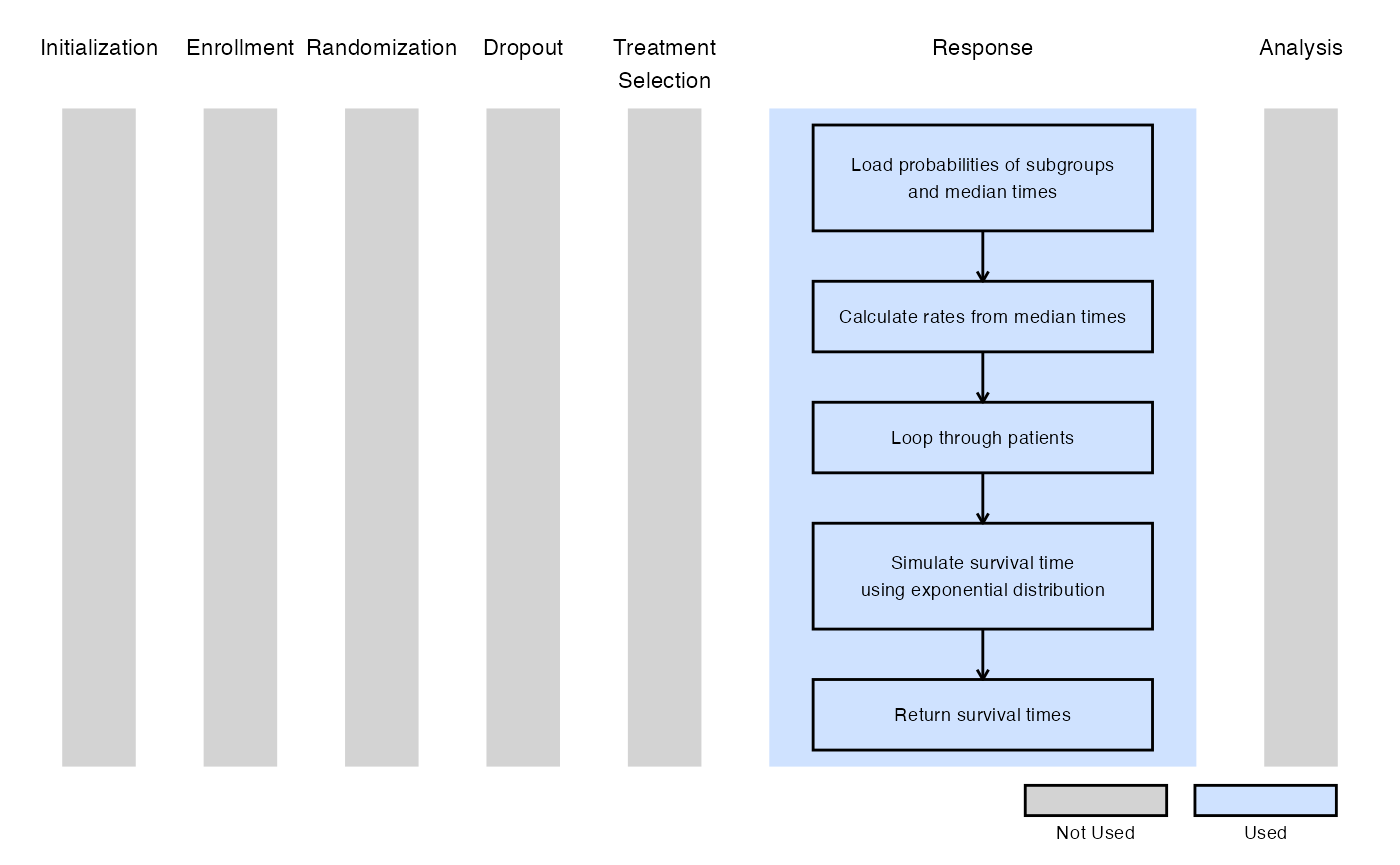
The figure below illustrates where this example fits within the R integration points of Cytel products, accompanied by a flowchart outlining the general steps performed by the R code.

Example 2.1 - No Group Difference

We are using two subgroups. Both subgroups have the same Hazard Ratio (HR), $HR = \frac{12}{16} = 0.75$ with same median TTE, i.e., subgroup has no impact. Refer to the table below for the values of the user-defined parameters used in this example.

User parameter	Value
QtyOfSubgroups	2
ProbSubgroup1	0.25
MedianTTECtrlSubgroup1	12
MedianTTEExpSubgroup1	16
ProbSubgroup2	0.75
MedianTTECtrlSubgroup2	12
MedianTTEExpSubgroup2	16

Example 2.2 - HR = 0.75

25% of patients are in subgroup 1, with a median TTE lower than in group 2. Both subgroups have an $HR = \frac{9}{12} = \frac{12}{16} = 0.75$ . Refer to the table below for the values of the user-defined parameters used in this example.

User parameter	Value
QtyOfSubgroups	2
ProbSubgroup1	0.25
MedianTTECtrlSubgroup1	9
MedianTTEExpSubgroup1	12
ProbSubgroup2	0.75
MedianTTECtrlSubgroup2	12
MedianTTEExpSubgroup2	16

Example 2.3 - Group 1 HR = 0.8 (Prob = 0.25), Group 2 HR = 0.75

25% of patients are in subgroup 1 with an $HR = \frac{9}{11.25} = 0.8$ . Subgroup 2 has an $HR = \frac{12}{16} = 0.75$ . Refer to the table below for the values of the user-defined parameters used in this example.

User parameter	Value
QtyOfSubgroups	2
ProbSubgroup1	0.25
MedianTTECtrlSubgroup1	9
MedianTTEExpSubgroup1	11.25
ProbSubgroup2	0.75
MedianTTECtrlSubgroup2	12
MedianTTEExpSubgroup2	16

Example 2.4 - Group 1 HR = 0.8 (Prob = 0.4), Group 2 HR = 0.75

40% of patients are in subgroup 1 with an $HR = \frac{9}{11.25} = 0.8$ . Subgroup 2 has an $HR = \frac{12}{16} = 0.75$ . Refer to the table below for the values of the user-defined parameters used in this example.

User parameter	Value
QtyOfSubgroups	2
ProbSubgroup1	0.4
MedianTTECtrlSubgroup1	9
MedianTTEExpSubgroup1	11.25
ProbSubgroup2	0.75
MedianTTECtrlSubgroup2	12
MedianTTEExpSubgroup2	16

The intent of the example is to illustrate the impact that the patient subgroup may have on the operating characteristics of the design.

Notes about the Exponential and Weibull Distributions

In R, the Weibull distribution is defined by a shape parameter $\alpha$ and a scale parameter $\sigma$ , with a probability density function (PDF) given by:

$f(x) = \frac{\alpha}{\sigma} \left(\frac{x}{\sigma}\right)^{\alpha-1} e^{-\left(\frac{x}{\sigma}\right)^\alpha}$

Its corresponding hazard function is:

$h(x) = \frac{\alpha}{\sigma} \left(\frac{x}{\sigma}\right)^{\alpha-1}$

The Exponential distribution in R is parameterized by a rate parameter $\lambda$ , with a PDF given by:

$f(x) = \lambda e^{-\lambda x}$

Its hazard function remains constant:

$h(x) = \lambda$

We can see that the Exponential distribution is a special case of the Weibull distribution, obtained by setting the shape parameter $\alpha = 1$ and the scale parameter $\sigma = \frac{1}{\lambda}$ .

Functions to assist in the computation of Weibull parameters can be found in HelperFunctionsWeibull.R.

2 Arm, Time-To-Event Outcome - Patient Simulation

Valeria A. G. Mazzanti, J. Kyle Wathen

June 04, 2025