2-Arm, Binary Outcome - Analysis

J. Kyle Wathen

January 16, 2025

Introduction

This example demonstrates how to add new analysis functionality into East using R functions.

For all examples, we assume the trial design consists of a control and an experimental treatment. There are 2 Interim Analyses (IA) and a Final Analysis (FA). At the IA, the analysis is performed and, depending on the example, may determine early efficacy or early futility depending on the design.

The examples included here are to provide different approaches for analyzing the data in the trial.

Once CyneRgy is installed, you can load this example in RStudio with the following commands:

CyneRgy::RunExample( "2ArmBinaryOutcomeAnalysis" )

Running the command above will load the RStudio project in RStudio.

East Workbook: 2ArmBinaryOutcomeAnalysis.cywx

RStudio Project File: 2ArmBinaryOutcomeAnalysis.Rproj

In the R directory of this example you will find the following R files:

1. AnalyzeUsingEastManualFormula.R - Contains a function named AnalyzeUsingEastManualFormula to demonstrate the R code necessary for this example as described below.

2. AnalyzeUsingPropTest.R - Contains a function named AnalyzeUsingPropTest to demonstrate the R code necessary for this example as described below.

3. AnalyzeUsingPropLimitsOfCI.R - Contains a function named AnalyzeUsingPropLimitsOfCI to demonstrate the R code necessary for this example as described below.

4. AnalyzeUsingBetaBinomial.R - Contains a function named AnalyzeUsingBetaBinomial to demonstrate the R code necessary for this example as described below.

In addition, if you would like to experiment with these examples to and would like some code to help you get started we have provided fill-in-the-blank type code files in the FillInTheBlankR directory.

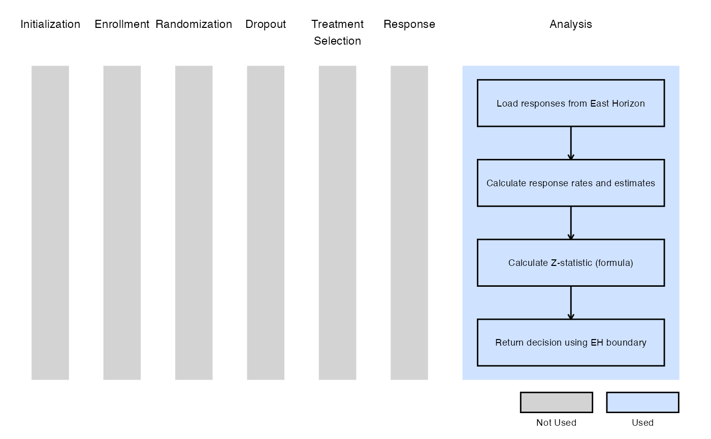
Example 1 - Two-Arm Binary Analysis Using Formula 28.2 in the East Manual

To replace the analysis, use the formula 28.2 in the East manual to compute the statistic. The purpose of this example is to demonstrate how the analysis and decision making could be modified in a simple approach. The test statistic is compared to the upper boundary computed and sent by East as an input. This example does NOT include a futility rule.

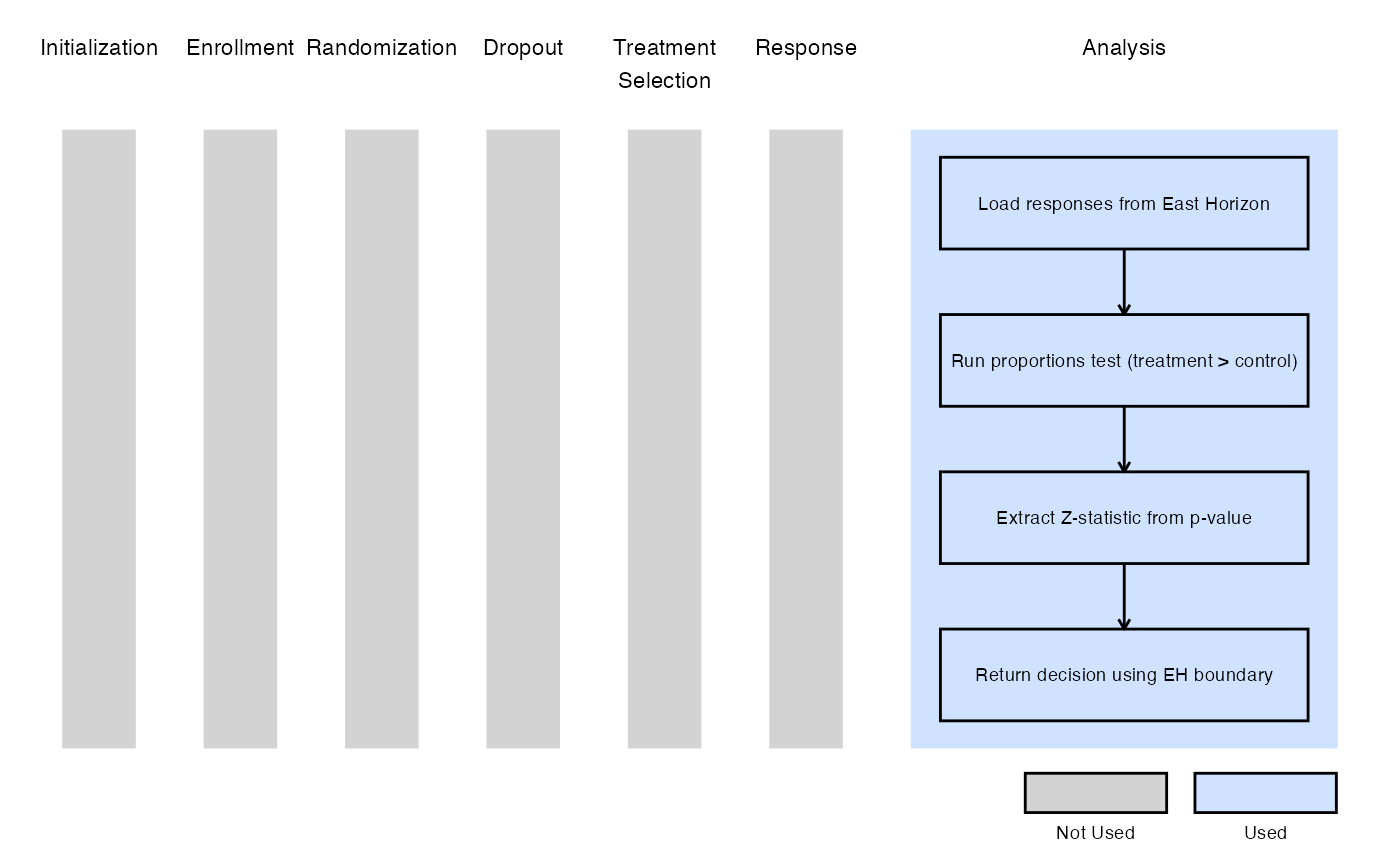
Example 2 - Two-Arm Binary Analysis Using the prop.test Function in Base R

This example utilizes the prop.test function in base R to perform the analysis. The p-value from prop.test is used to compute the Z statistic that is compared to the upper boundary computed and sent by East as an input. This example does NOT include a futility rule.

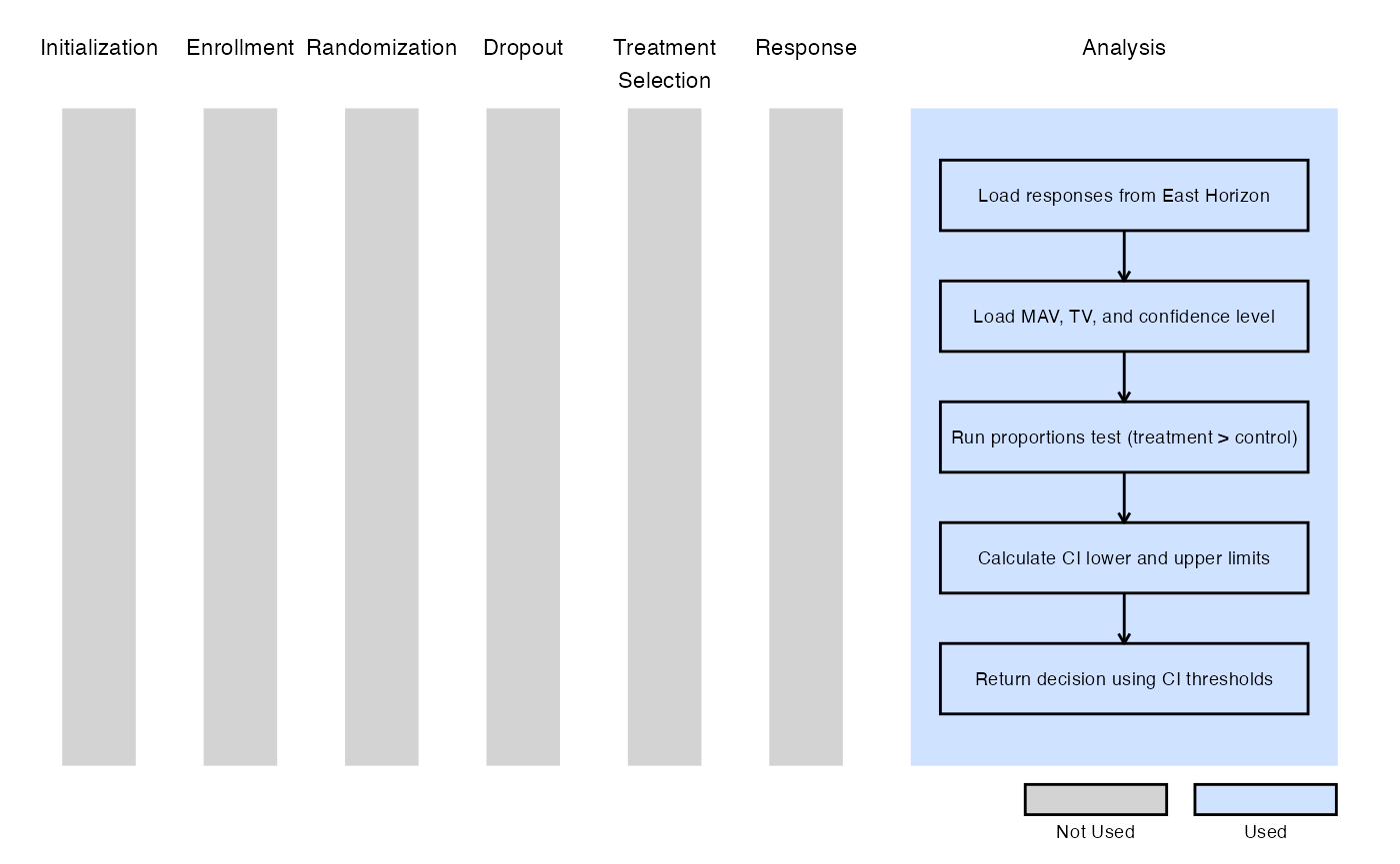
Example 3 - Utilization of Confidence Interval Limits for Go/No-Go Decision Making

In many phase II trials, teams like to utilize the upper and lower boundaries of a confidence interval (CI) for making Go and No-Go type decision. In this type of trial, teams often set a Minimum Acceptable Value (MAV), the minimum treatment difference that would warrant further development in a product, and a Target Value (TV), the value that is highly desirable based on other consideration. In this simplified example, if it is likely that the treatment difference is above the MAV then a Go decision is made. If a Go decision is not made, then if it is unlikely that the treatment difference is above the TV, a No-Go decision is made.

In this example, the prop.test from base R is utilized to analyze the data and compute a user-specified confidence interval. If user-specified variables are not defined, we assume the MAV = 0.1 and TV = 0.2. The team would like to make a Go decision if there is at least a 90% chance that the difference in treatment is greater than the MAV. If a Go decision is not made, then a No-Go decision is made if there is less than a 10% chance the difference is greater than the TV. Using a frequentist CI an approximation to this design can be done by the logic described below.

At an Interim Analysis

• If the Lower Limit of the CI (LL) is greater than a user-specified amount then a Go decision is made. Specifically, if LL > user-specified lower limit –> Go.
• If a Go decision is not made, then if the Upper Limit of the CI (UL) is less than a user-specified value a No-Go decision is made. Specifically, if UL < user-specified upper limit –> No-Go.
• Otherwise, continue to the next analysis.

At the Final Analysis

• If the Lower Limit of the CI, denoted by LL, is greater than a user-specified values then a Go decision is made. Specifically, if LL > user-specified value –> Go.
• Otherwise, a No-Go decision is made.

Note, in this example the boundary information that is computed and sent from East is ignored in order to implement this decision approach.

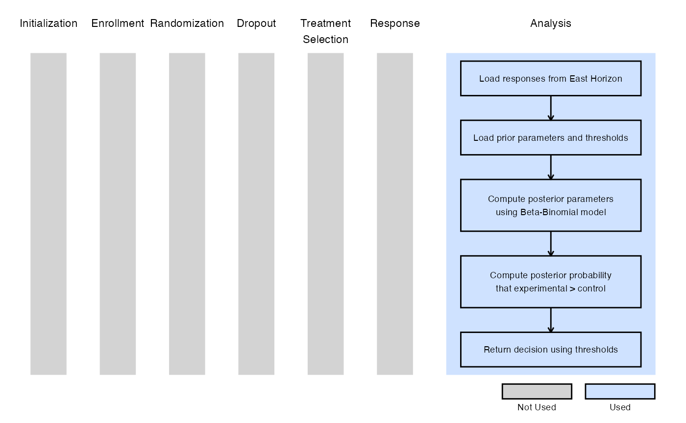
Example 4 - Bayesian Analysis

In this example, the default values of user-specified variables utilize prior data on 50 patients and incorporate the data directly into the Bayesian model. The Beta distributions for both standard of care and experimental as well as the upper limit for efficacy and lower limit for futility can be user-specified variables. With the default user-specified values in the prior data, 10 patients had a response and 40 patients had a treatment failure. Denote the response rate for standard of care by $\pi_S$ and on experimental by $\pi_E$ and we assume the following prior distributions:

$\pi_S \sim$ Beta( 10, 40 ) which has a prior mean response rate of 20% and is equivalent to observing 50 prior patients with 10 responses.

$\pi_E \sim$ Beta( 0.2, 0.8 ) which has a prior mean response rate of 20% and is equivalent to observing 1 prior patient.

The Beta distribution is conjugate for binary data. Assuming $N_{Ctrl}$ and $N_{Exp}$ patients have enrolled on Control (Ctrl) and Experimental (Exp), respectively, the following data are observed at an interim analysis:

Treatment	Number of Responses	Number of Treatment Failures
Ctrl	$X_{Ctrl}$	$N_{Ctrl} - X_{Ctrl}$
Exp	$X_{Exp}$	$N_{Exp} - X_{Exp}$

Then posterior distributions are:

$\pi_{Ctrl} | N_{Ctrl}, X_{Ctrl} \sim$ Beta( 10 + $X_{Ctrl}$, 40 + $N_{Ctrl} - X_{Ctrl}$ )

$\pi_{Ctrl} | N_{Exp}, X_{Exp} \sim$ Beta( 0.2 + $X_{Exp}$, 0.8 + $N_{Exp} - X_{Exp}$ )

For analysis and decision making, the posterior distributions are used to stop the trial for efficacy if it is very likely that the response rate on E is higher than on S and stop for futility if it is unlikely that the response rate on E is better than S. Specifically, compute the posterior probability that E has a higher response rate than S:

$\rho = Pr( \pi_{Exp} > \pi_{Ctrl} | X_{Ctrl}, N_{Ctrl}, X_{Exp}, N_{Exp} )$

At the Interim Analysis

• If $\rho > 0.975$ then make an early efficacy (Go) decision
• If $\rho < 0.10$ then make an early futility (No-Go) decision.

Note that the above values can be user-specified.

At the Final Analysis

• If $\rho > 0.95$ make an efficacy decision, otherwise a futility decision is made.

This example demonstrates how prior data and an informative prior on $\pi_S$ can impact decision making. However, a full sensitivity analysis to the prior information and impact on Operating characteristics should be explored with approaches like this.