Consecutive Studies, Continuous Outcome

The following scripts are related to the Integration Point: Analysis and the Integration Point: Response. Click on the links for more information about these integration points.

The following example does not show how to load Phase 2 data into a Phase 3 trial. Please see the Consecutive Studies, Binary Outcome example for more information and step-by-step instructions.

Introduction

The intent of the following example is to demonstrate the computation of Bayesian assurance, or probability of success, and conditional assurance in consecutive studies by using custom R scripts for the Response (Patient Simulation) and the Analysis integration points of East Horizon. It features a sequential design involving a Phase 2 trial followed by a Phase 3 trial, both with continuous outcomes.

The objective is to understand how conducting a Phase 2 study can reduce the risk associated with the Phase 3 trial. This de-risking is evaluated by comparing two scenarios: (1) the probability of a No-Go decision in Phase 3 if Phase 2 is skipped, and (2) the probability of a No-Go in Phase 3 if a preceding Phase 2 trial is conducted and yields a Go decision. Specifically, we compute the conditional assurance of Phase 3 given success in Phase 2.

The scenarios covered are as follows:

Two consecutive studies: phase 2 with a normal endpoint followed by phase 3, also with a normal endpoint.

Once CyneRgy is installed, you can load this example in RStudio with the following commands:

CyneRgy::RunExample( "ConsecutiveStudiesContinuous" )

Running the command above will load the RStudio project in RStudio.

In the R directory of this example you will find the R files used in the examples:

SimulatePatientOutcomeNormalAssurance.R - Functions to simulate patient outcomes under a normal distribution informed by mixture priors.
AnalyzeUsingBayesianNormals.R - Implements Bayesian analysis of simulated outcomes using normal priors.

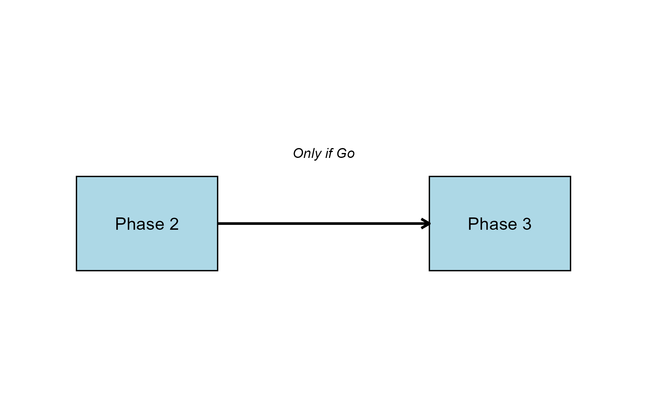
Note: This example builds on the Bayesian Assurance, Continuous Outcome example, and utilizes the same R code. Please refer to it for more information. The difference is that we now have two different studies: Phase 3 is conducted only if Phase 2 results in a Go decision.

Phase 2 Study

This study considers a two-arm fixed sample design with normally distributed outcomes $Y$ , with 80 patients per treatment arm.

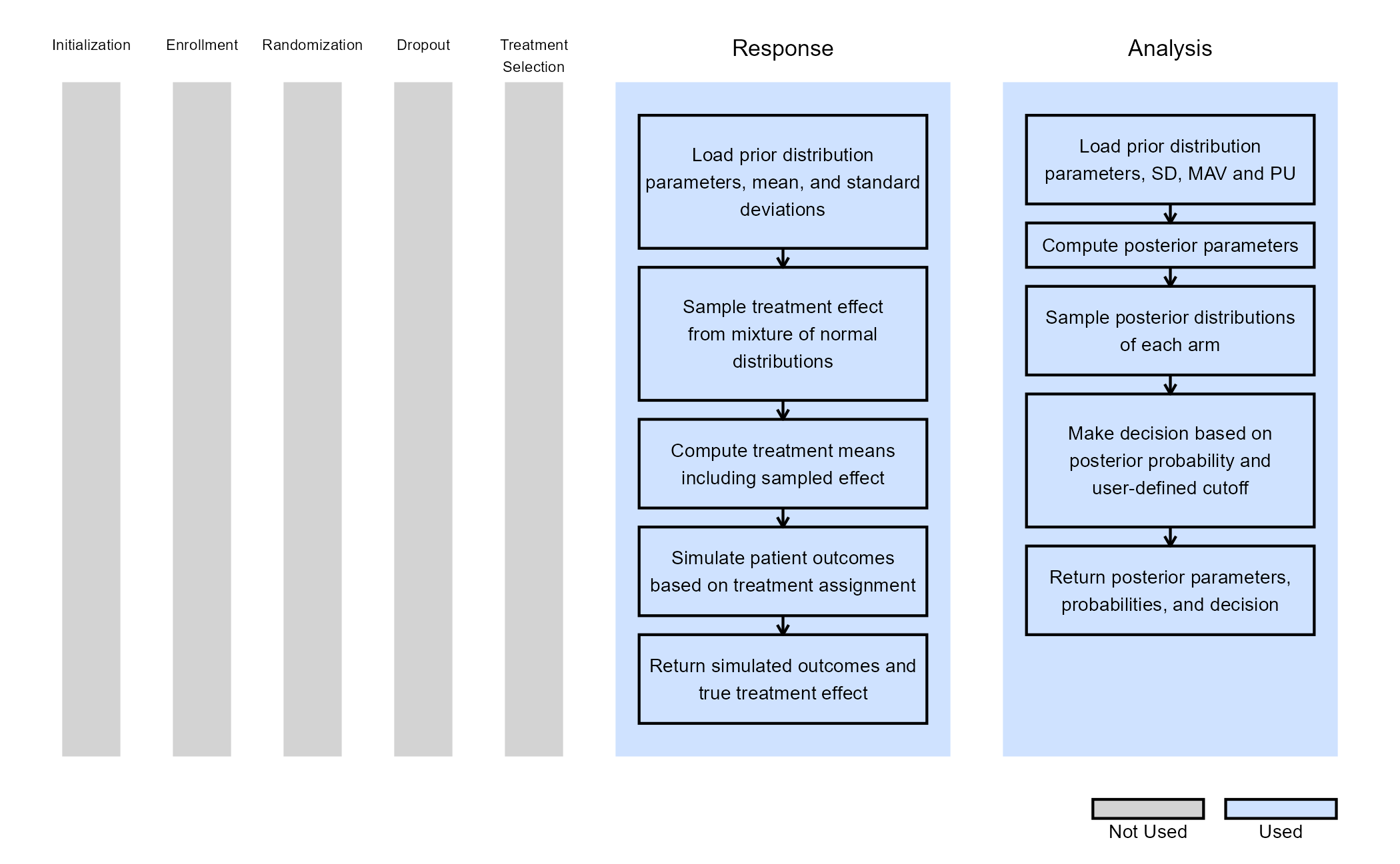
The figure below illustrates where this phase fits within the R integration points of Cytel products, accompanied by flowcharts outlining the general steps performed by the R code.

Response (Patient Simulation) Integration Point

This endpoint is related to this R file: SimulatePatientOutcomeNormalAssurance.R

This function simulates patient-level outcomes within a Bayesian assurance framework, using a two-component mixture prior to reflect uncertainty about the true treatment effect. It allows for assessing the probability of trial success (assurance) under uncertainty about the true treatment effect. Information generated from this simulation will be used later for the Analysis Integration Point.

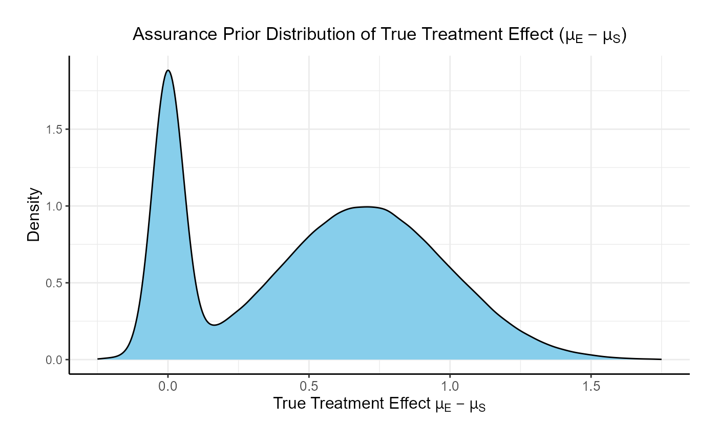
In this example, the true treatment effect ( $\mu_E - \mu_S$ ) is sampled from a mixture of two normal priors:

25% weight on $\mathcal{N}(0, 0.05^2)$ .
75% weight on $\mathcal{N}(0.7, 0.3^2)$ .

The control mean is fixed, while the experimental mean is computed as $d\text{MeanCtrl} + \text{treatment effect}$ . Each patient’s response is then simulated from a normal distribution corresponding to their assigned treatment group, with standard deviations defined separately for each arm.

Refer to the table below for the definitions and values of the user-defined parameters used in this example.

User parameter	Definition	Value
dWeight1	Weight of prior component 1.	0.25
dWeight2	Weight of prior component 2.	0.75
dMean1	Mean of prior component 1.	0
dMean2	Mean of prior component 2.	0.7
dSD1	Standard deviation of prior component 1.	0.05
dSD2	Standard deviation of prior component 2.	0.3
dMeanCtrl	Mean of control arm (experimental arm will be sampled).	0
dSDCtrl	Standard deviation for control arm.	1.9
dSDExp	Standard deviation for experimental arm.	1.9

Analysis Integration Point

This endpoint is related to this R file: AnalyzeUsingBayesianNormals.R

This function evaluates the posterior probability that the experimental treatment arm is better than the control arm by more than a clinically meaningful threshold, and returns a Go/No-Go decision based on a cutoff ( $P_U$ ). It uses information from the simulation that is generated by the Response element of East Horizon’s simulation, explained above.

For patients receiving treatment $j \in \{\text{S}, \text{E}\}$ (S = standard/control, E = experimental), we assume the outcomes $Y \sim \mathcal{N}(\mu_j, \sigma^2)$ , where $\mu_j$ is an unknown mean and $\sigma^2$ is a known, fixed variance.

We assume a priori that:

$\mu_j \sim \mathcal{N}(\theta_j, \tau_j^2 = 1000^2), \quad j \in \{\text{S}, \text{E}\}$

After observing $n$ patients on treatment $j$ , the posterior distribution of $\mu_j$ becomes:

$\mu_j \mid \bar{y} \sim \mathcal{N}(\theta_j^*, \tau_j^{2*})$

where:

$\theta_j^* = \frac{\frac{\theta_j}{\tau_j^2} + \frac{n \bar{y}}{\sigma^2}}{\frac{1}{\tau_j^2} + \frac{n}{\sigma^2}}, \quad \text{and} \quad \frac{1}{\tau_j^{2*}} = \frac{1}{\tau_j^2} + \frac{n}{\sigma^2}$

At the conclusion of the study, the posterior probability that the experimental arm exceeds the control arm by more than the minimum acceptable value (MAV) is calculated as:

$\rho = \Pr(\mu_E > \mu_S + \text{MAV} \mid \text{data})$

The decision rule is as follows:

If $\rho > P_U \rightarrow$ Go.
If $\rho \leq P_U \rightarrow$ No-Go.

For this study, the MAV is set to 0.6 and $P_U$ to 0.8. Refer to the table below for all the definitions and values of the user-defined parameters used in this example.

User parameter	Definition	Value
dPriorMeanCtrl	Prior mean for control arm.	0
dPriorStdDevCtrl	Prior standard deviation for control arm.	1000
dPriorMeanExp	Prior mean for experimental arm.	0
dPriorStdDevExp	Prior standard deviation for experimental arm.	1000
dSigma	Known sampling standard deviation.	1.9
dMAV	Minimum Acceptable Value (clinically meaningful difference).	0.6
dPU	Go threshold (posterior probability cutoff).	0.8

Phase 3 Study

This study considers a two-arm fixed sample design with normally distributed outcomes $Y$ , with 200 patients per treatment arm.

The figure below illustrates where this phase fits within the R integration points of Cytel products, accompanied by flowcharts outlining the general steps performed by the R code.

Response (Patient Simulation) Integration Point

This endpoint is related to this R file: SimulatePatientOutcomeNormalAssurance.R

The function for the Response Integration Point of the Phase 3 Study is the same as in Phase 2. Refer to the table below for the definitions and values of the user-defined parameters used in this example.

User parameter	Definition	Value
dWeight1	Weight of prior component 1.	0.25
dWeight2	Weight of prior component 2.	0.75
dMean1	Mean of prior component 1.	0
dMean2	Mean of prior component 2.	0.7
dSD1	Standard deviation of prior component 1.	0.05
dSD2	Standard deviation of prior component 2.	0.3
dMeanCtrl	Mean of control arm (experimental arm will be sampled).	0
dSDCtrl	Standard deviation for control arm.	1.9
dSDExp	Standard deviation for experimental arm.	1.9

Analysis Integration Point

This endpoint is related to this R file: AnalyzeUsingBayesianNormals.R

The function for the Analysis Integration Point of the Phase 3 Study is the same as in Phase 2.

However, for this study, the MAV is set to 0.6 and $P_U$ to 0.5. This design is equivalent to a t-test because the critical value would be 0.6 and having a posterior probability greater than 0.5 would indicate that the estimated treatment difference is above the critical value.

Refer to the table below for all the definitions and values of the user-defined parameters used in this example.

User parameter	Definition	Value
dPriorMeanCtrl	Prior mean for control arm.	0
dPriorStdDevCtrl	Prior standard deviation for control arm.	1000
dPriorMeanExp	Prior mean for experimental arm.	0
dPriorStdDevExp	Prior standard deviation for experimental arm.	1000
dSigma	Known sampling standard deviation.	1.9
dMAV	Minimum Acceptable Value (clinically meaningful difference).	0.6
dPU	Go threshold (posterior probability cutoff).	0.5

Results

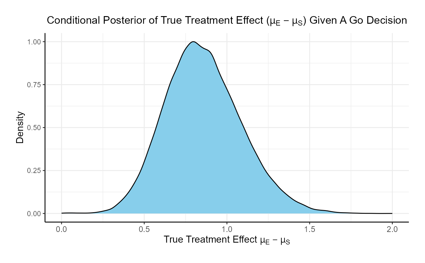
For the phase 2 study independently, the probability of a Go is 26.7% and the probability of a No-Go is 73.3%.

For the phase 3 study independently, the probability of a Go is 46% and the probability of a No-Go is 54%.

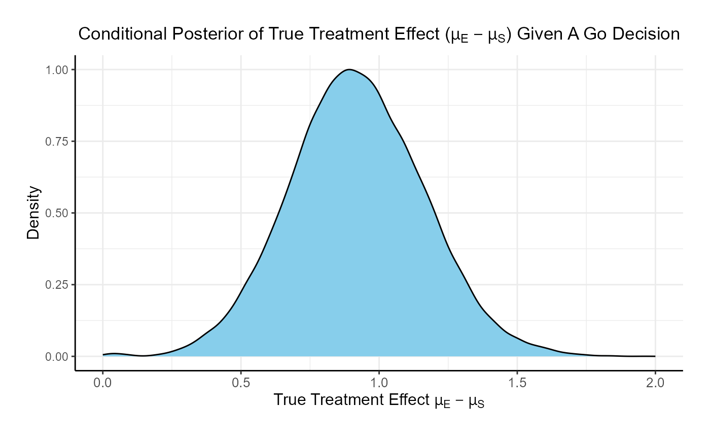
If the two studies are run sequentially, conducting Phase 3 only if Phase 2 results in a Go decision, the probability of a Go in Phase 3 is 84.8% and the probability of a No-Go is 15.2%.

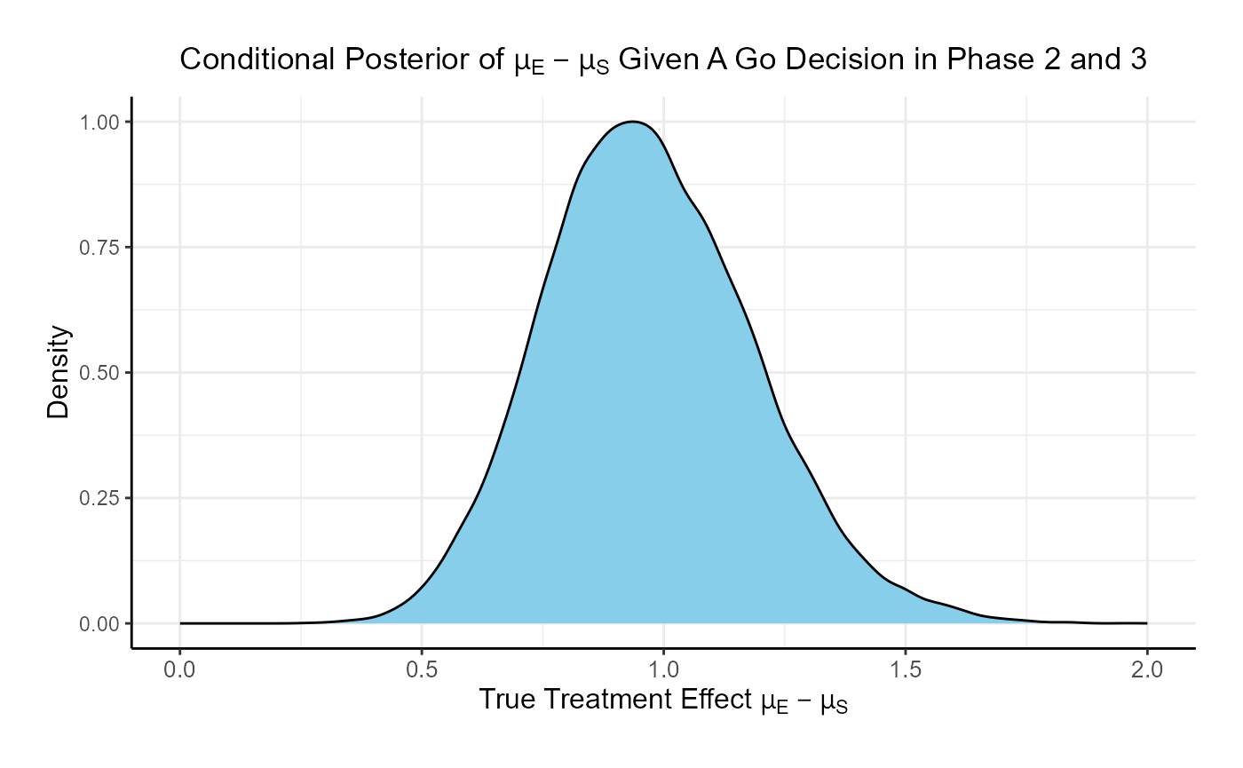
Comparing the option of running only a Phase 3 versus a Phase 2 followed by a Phase 3 if Phase 2 is successful, the probability of Go in phase 3 increases from 46% to 84.8% and the probability of a No-Go in Phase 3 decreases from 54% to 15.2%.

J. Kyle Wathen and Laurent Spiess

October 16, 2025

Introduction

Phase 2 Study

Response (Patient Simulation) Integration Point

Analysis Integration Point

Phase 3 Study

Response (Patient Simulation) Integration Point

Analysis Integration Point

Results

See Also