Bayesian Assurance, Time-to-Event Outcome
J. Kyle Wathen and Laurent Spiess
July 07, 2026
BayesianAssuranceTimeToEvent.RmdThis example is related to both the Integration Point: Response - Time-to-Event Outcome and the Integration Point: Analysis - Time-to-Event Outcome. Click the links for setup instructions, variable details, and additional information about the integration points.
- Study objective: Two Arm Confirmatory
- Number of endpoints: Single Endpoint
- Endpoint type: Time-to-Event Outcome
- Task: Explore
Note: This example is compatible with both Fixed Sample and Group Sequential statistical designs. The R code automatically detects whether interim look information (LookInfo) is available and adjusts the analysis parameters accordingly.
Introduction
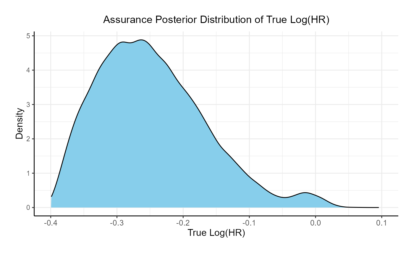
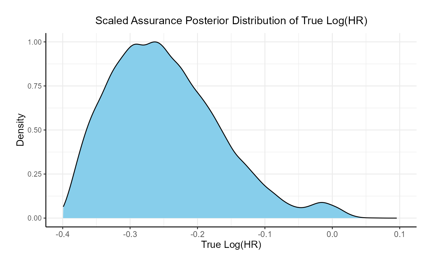
The intent of the following example is to demonstrate the computation of Bayesian assurance, or probability of success, through the integration of R with Cytel products. The example features a two-arm trial with time-to-event outcome, using a bi-modal distribution prior to compute assurance.
The scenario covered is as follows:
- Fixed sample design using a bi-modal distribution and Cox proportional hazards model to compute Bayesian assurance.
Once CyneRgy is installed, you can load this example in RStudio with the following command:
CyneRgy::RunExample( "BayesianAssuranceTimeToEvent" )Running the command above will load the RStudio project in RStudio.
In the R directory of this example you will find the R files used in the examples:
- SimulatePatientSurvivalAssurance.R - Functions to simulate patient outcomes under a time-to-event distribution informed by a bi-modal prior.
- AnalyzeSurvivalDataUsingCoxPH.R - Implements Bayesian analysis of simulated outcomes using Cox proportional hazards model.
Example 1 - Fixed Sample Design
This example considers a two-arm fixed sample design with a time-to-event endpoint, with 300 patients per arm. It demonstrates how to customize the the Response (Patient Simulation) element of East Horizon’s simulation to simulate the true hazard ratio from the prior and then simulate the patient data using the sampled hazard ratio, and the Analysis element of East Horizon’s simulation to perform the analysis using a Cox model.
The figure below illustrates where this example fits within the R integration points of Cytel products, accompanied by flowcharts outlining the general steps performed by the R code.
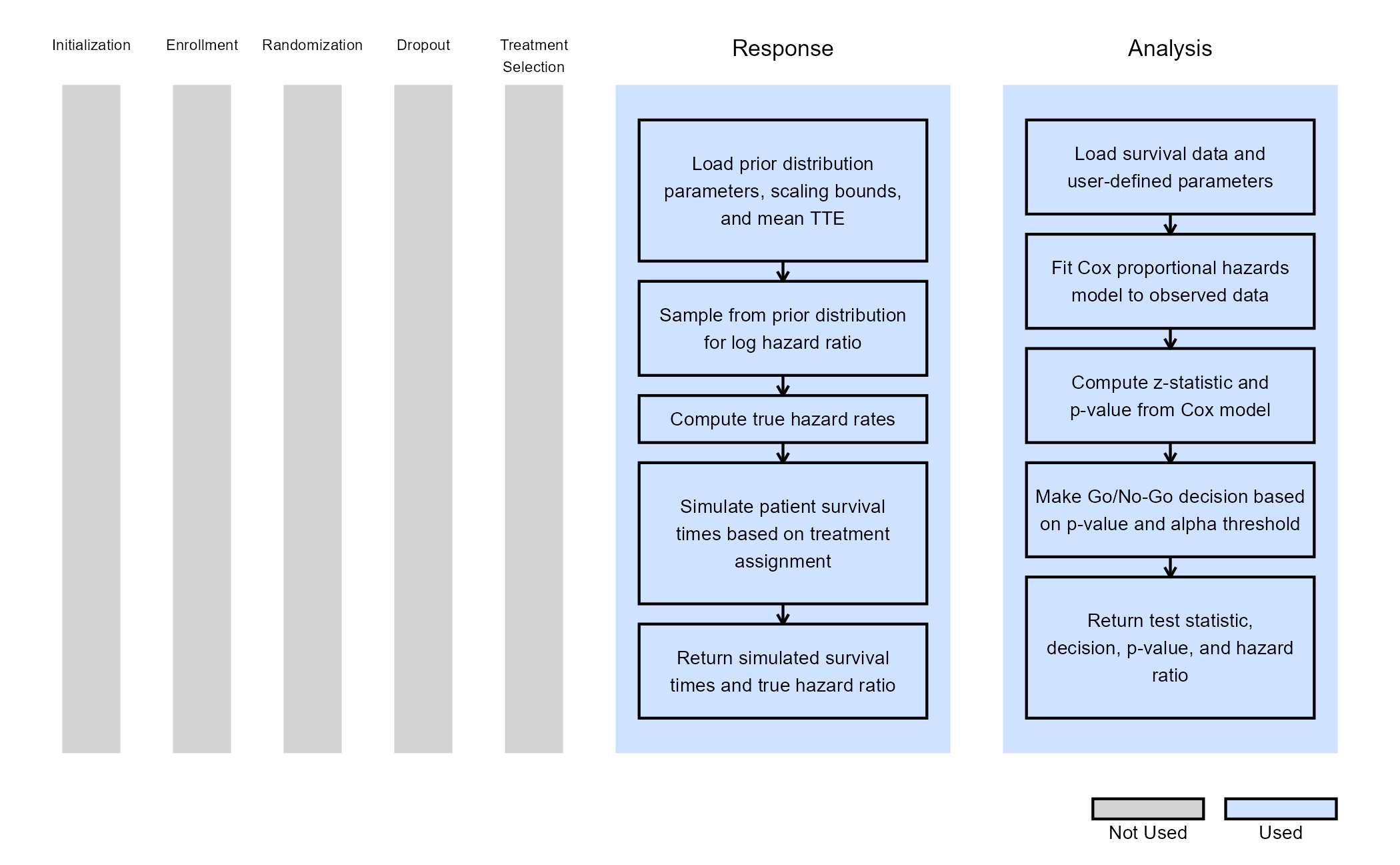
Response (Patient Simulation) Integration Point
This endpoint is related to this R file: SimulatePatientSurvivalAssurance.R
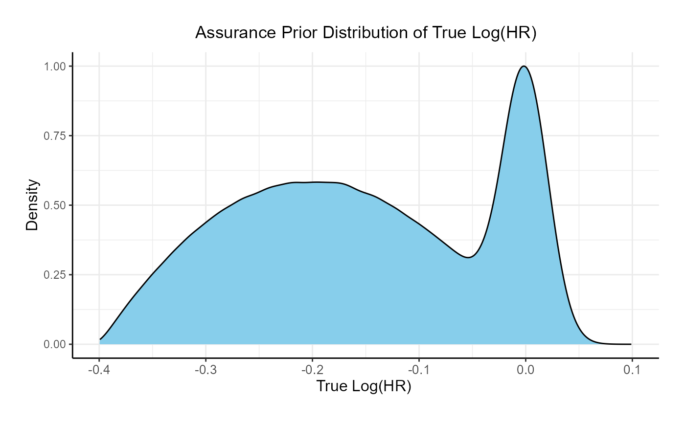
This function simulates patient-level outcomes within a Bayesian assurance framework. Information generated from this simulation will be used later for the Analysis Integration Point. In this example, a bi-modal prior on the is used. The components of the prior are:
- 25% weight on .
- 75% weight on , rescaled between -0.4 and 0.
Refer to the table below for the definitions and values of the user-defined parameters used in this example.
| User parameter | Definition | Value |
|---|---|---|
| dWeight1 | Probability of using the normal prior for log(HR). | 0.25 |
| dPriorMean | Mean of the normal prior for log(HR). | 0 |
| dPriorSD | Standard deviation of the normal prior for log(HR). | 0.02 |
| dAlpha | Alpha parameter of the Beta prior for log(HR). | 2 |
| dBeta | Beta parameter of the Beta prior for log(HR). | 2 |
| dUpper | Upper bound for scaling the Beta prior. | 0 |
| dLower | Lower bound for scaling the Beta prior. | -0.4 |
| dMeanTTEControl | Mean time-to-event for the control group. | 12 |
Analysis Integration Point
This endpoint is related to this R file: AnalyzeSurvivalDataUsingCoxPH.R
A single analysis is conducted once 50% of patients have experienced the event of interest. Using the function in the file, the analysis employs a Cox proportional hazards model, with a hazard ratio (HR) less than 1 indicating a benefit in favor of the experimental arm. It uses information from the simulation that is generated by the Response element of East Horizon’s simulation, explained above. A Go decision is made if the resulting p-value is less than or equal to 0.025. Refer to the table below for the definitions of the user-defined parameters used in this example.
| User parameter | Definition |
|---|---|
| bReturnLogTrueHazard | If True, the function returns the natural logarithm of
the true hazard ratio instead of its raw value. |
| bReturnNAForNoGoTrials | If True and the trial does not meet the Go decision
criterion, the function returns NA for the hazard
ratio. |