Multiple Arm, Patient Simulation
Gabriel Potvin and Anoop Singh Rawat
September 17, 2026
MultiArmPatientSimulation.RmdThis example is related to the Integration Point: Response. Click the link for setup instructions, variable details, and additional information about this integration point.
- Study objective: Multiple Arm Confirmatory, 3 Arms
- Number of endpoints: Single Endpoint
- Endpoint type:
- Continuous Outcome for Example 1
- Binary Outcome for Example 2
- Time-to-Event Outcome for Example 3 and 4
- Task: Explore or Design
Introduction
The following examples illustrate how to integrate new patient outcome simulation (response) capabilities into East Horizon using R functions in the context of a multi-arm clinical trials. The following examples demonstrate different approaches for simulating continuous, binary, and time-to-event endpoints in multi-arm clinical trials.
Once CyneRgy is installed, you can load this example in RStudio, VS Code, or any other supported IDE with the following command:
CyneRgy::RunExample( "MultiArmPatientSimulation" )In the R directory of this example you will find the following R files:
SimulatePatientOutcomeMultiArmPercentAtZero.R - Simulates continuous outcomes from a mixture distribution where a proportion of patients have no response.
SimulatePatientOutcomeMultiArmPercentAtZero.Binary.R - Simulates binary outcomes from a mixture distribution where a proportion of patients have no response.
SimulatePatientSurvivalMultiArmWeibull.R - Simulates time-to-event outcomes using a Weibull distribution, allowing arm-specific shape and scale parameters.
SimulatePatientSurvivalMultiArmExpGivenMST.R - Simulates time-to-event outcomes using exponential survival distributions specified through arm-specific median survival times.
Example 1 - Simulation of Continuous Outcomes with Non-Responders
This example is related to this R file: SimulatePatientOutcomeMultiArmPercentAtZero.R
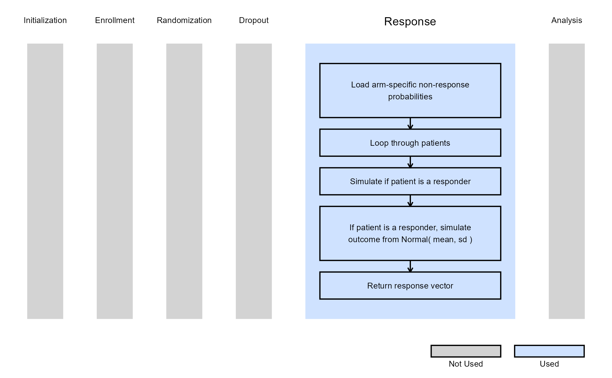
In this example, each patient’s outcome represents a change from baseline. However, some patients are expected to show no improvement (non-responders), leading to an outcome of zero. The proportion of such patients can vary across treatment arms (e.g., between 20% and 40% based on prior data).
The function SimulatePatientOutcomeMultiArmPercentAtZero extends the two-arm approach to three arms (two treatment arms), simulating each patient’s outcome according to their assigned treatment. For each arm, the function uses the probability of a zero outcome to determine whether a patient is a non-responder; responders then have their outcome simulated from a normal distribution with arm-specific mean and standard deviation.
Note: This example could be extended to any number
of treatment arms by adding more user parameters such as
dProbOfZeroOutcomeExp3,
dProbOfZeroOutcomeExp4, etc.
Refer to the table below for the definitions of the user-defined parameters used in this example.
| User parameter | Definition |
|---|---|
| dProbOfZeroOutcomeCtrl | Value between 0 and 1 representing the probability a patient is a non-responder in the control arm. |
| dProbOfZeroOutcomeExp1 | Value between 0 and 1 representing the probability a patient is a non-responder in the first experimental arm. |
| dProbOfZeroOutcomeExp2 | Value between 0 and 1 representing the probability a patient is a non-responder in the second experimental arm. |
The figure below illustrates where this example fits within the R integration points of Cytel products, accompanied by a flowchart outlining the general steps performed by the R code.
Example 2 - Simulation of Binary Outcomes with Treatment Resistance
This example is related to this R file: SimulatePatientOutcomeMultiArmPercentAtZero.Binary.R
In this example, patient outcomes are binary, where 0
represents treatment failure (non-response), and 1
indicates a successful treatment and response. Some patients, however,
are treatment-resistant, meaning they will not respond to any treatment
and thus always yield an outcome of 0. The proportion of
resistant patients can differ between treatment arms.
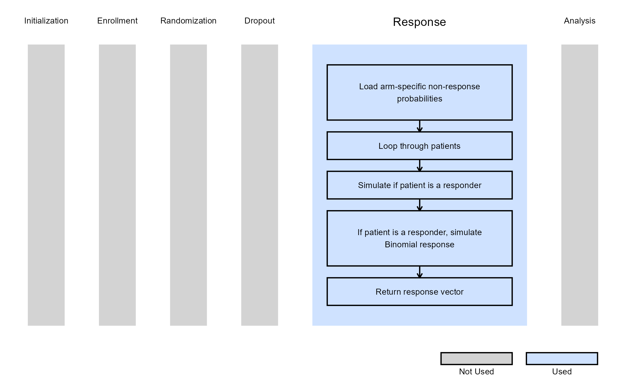
The R function SimulatePatientOutcomeMultiArmPercentAtZero.Binary extends the two-arm approach to three arms (two treatment arms), where each arm has its own probability of treatment resistance. For each simulated patient, the function first determines whether they are treatment-resistant and, if not, simulates their binary response using the arm-specific probability of success.
Note: This example could be extended to any number
of treatment arms by adding more user parameters such as
dProbOfTreatmentResistantExp3,
dProbOfTreatmentResistantExp4, etc.
Refer to the table below for the definitions of the user-defined parameters used in this example.
| User parameter | Definition |
|---|---|
| dProbOfTreatmentResistantCtrl | Value between 0 and 1 representing the probability a patient is treatment-resistant in the control arm. |
| dProbOfTreatmentResistantExp1 | Value between 0 and 1 representing the probability a patient is treatment-resistant in the first experimental arm. |
| dProbOfTreatmentResistantExp2 | Value between 0 and 1 representing the probability a patient is treatment-resistant in the second experimental arm. |
The figure below illustrates where this example fits within the R integration points of Cytel products, accompanied by a flowchart outlining the general steps performed by the R code.
Example 3 - Simulation of Time-to-Event Outcomes from a Weibull Distribution
This example is related to this R file: SimulatePatientSurvivalMultiArmWeibull.R
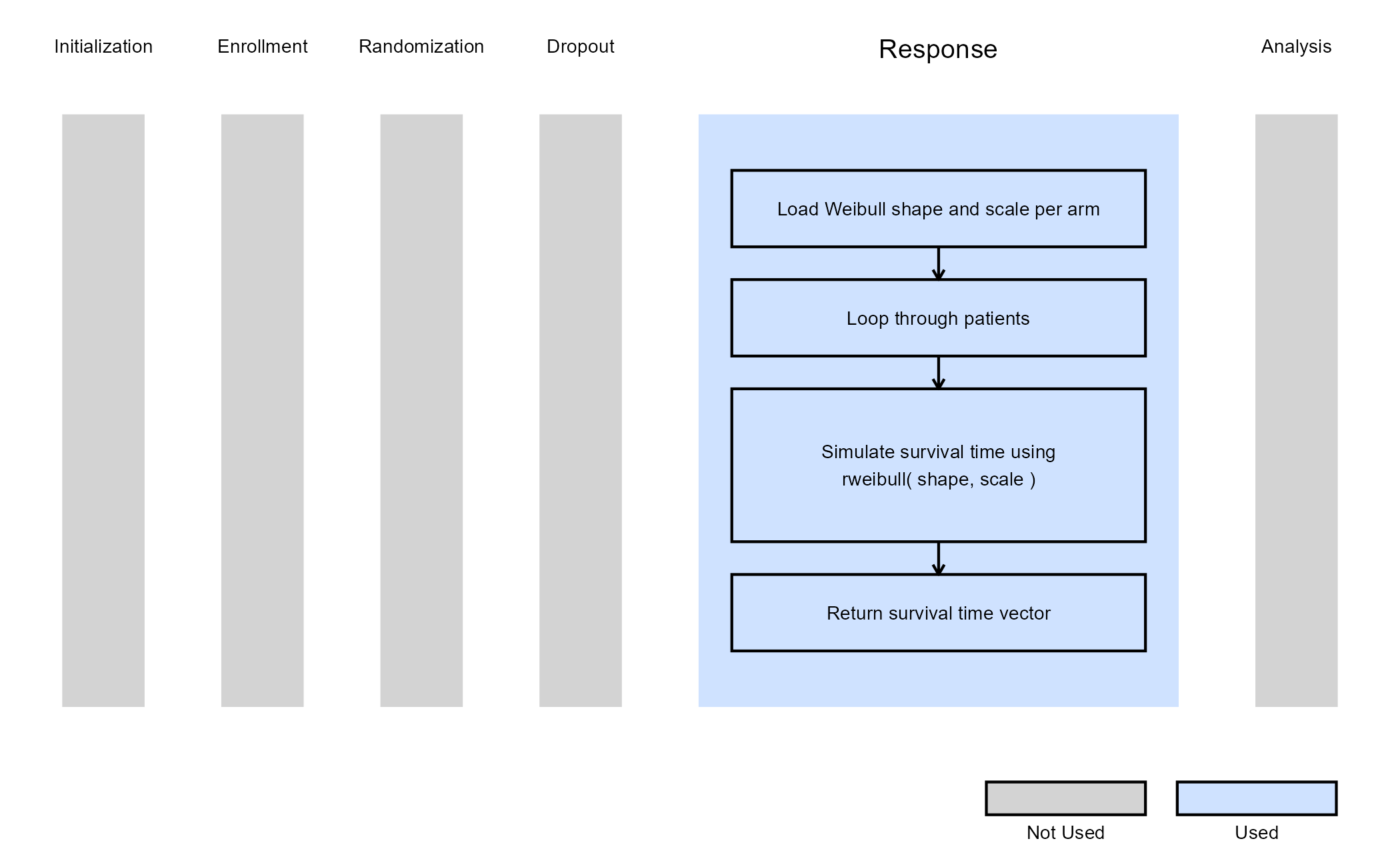
This example demonstrates how to simulate time-to-event data for multiple treatment arms using arm-specific Weibull parameters. Each arm is characterized by its own shape and scale values, allowing flexible modeling of distinct hazard profiles across arms.
The R function SimulatePatientSurvivalMultiArmWeibull extends the two-arm approach to three arms (two treatment arms), generating a survival time for each patient according to the Weibull distribution corresponding to their assigned arm. This enables users to evaluate study power or expected treatment differences under non-proportional hazards or complex multi-arm designs.
Note: This example could be extended to any number
of treatment arms by adding more user parameters such as
dShapeExp3 and dScaleExp3,
dShapeExp4 and dScaleExp4, etc.
Refer to the table below for the definitions of the user-defined parameters used in this example.
| User parameter | Definition |
|---|---|
| dShapeCtrl | Shape parameter of the Weibull distribution for the control arm. |
| dShapeExp1 | Shape parameter of the Weibull distribution for the first experimental arm. |
| dShapeExp2 | Shape parameter of the Weibull distribution for the second experimental arm. |
| dScaleCtrl | Scale parameter of the Weibull distribution for the control arm. |
| dScaleExp1 | Scale parameter of the Weibull distribution for the first experimental arm. |
| dScaleExp2 | Scale parameter of the Weibull distribution for the second experimental arm. |
The figure below illustrates where this example fits within the R integration points of Cytel products, accompanied by a flowchart outlining the general steps performed by the R code.
Example 4 - Simulation of Time-to-Event Outcomes from Median Survival Times
This example is related to this R file: SimulatePatientSurvivalMultiArmExpGivenMST.R
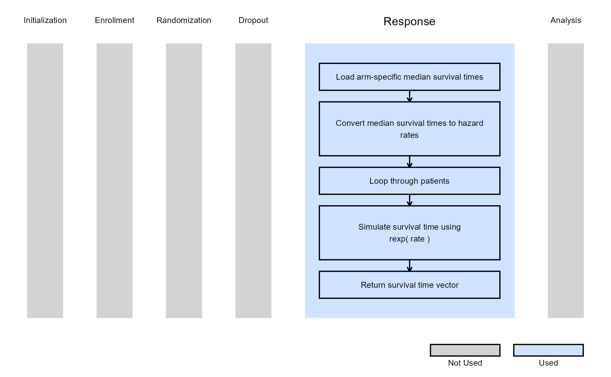
This example demonstrates how to simulate time-to-event outcomes for multiple treatment arms using arm-specific median survival times (MSTs). Rather than requiring hazard rates directly, the function accepts the median survival time for each treatment arm, internally converts each value into an exponential hazard rate using and then generates survival times from exponential distributions.
The R function SimulatePatientSurvivalMultiArmExpGivenMST extends the multi-arm survival simulation framework by allowing users to specify clinically interpretable median survival times (from East Horizon) instead of hazard rates. Each patient’s treatment assignment determines which exponential distribution is used for simulation.
Note: This example currently supports exponential
survival models based on median survival times
(SurvMethod = 3). It can easily be extended to additional
treatment arms by supplying additional median survival time values.
The figure below illustrates where this example fits within the R integration points of Cytel products, accompanied by a flowchart outlining the general steps performed by the R code.